6 Débrief : compléments d’information
6.1 Le point sur les jointures
library("dplyr")Jointure à gauche, à droite, interne ou complète ? (rappel théorique)
band_members# A tibble: 3 x 2
name band
<chr> <chr>
1 Mick Stones
2 John Beatles
3 Paul Beatlesband_instruments# A tibble: 3 x 2
name plays
<chr> <chr>
1 John guitar
2 Paul bass
3 Keith guitarleft_join(band_members, band_instruments)Joining, by = "name"# A tibble: 3 x 3
name band plays
<chr> <chr> <chr>
1 Mick Stones <NA>
2 John Beatles guitar
3 Paul Beatles bass right_join(band_members, band_instruments)Joining, by = "name"# A tibble: 3 x 3
name band plays
<chr> <chr> <chr>
1 John Beatles guitar
2 Paul Beatles bass
3 Keith <NA> guitarinner_join(band_members, band_instruments)Joining, by = "name"# A tibble: 2 x 3
name band plays
<chr> <chr> <chr>
1 John Beatles guitar
2 Paul Beatles bass full_join(band_members, band_instruments)Joining, by = "name"# A tibble: 4 x 3
name band plays
<chr> <chr> <chr>
1 Mick Stones <NA>
2 John Beatles guitar
3 Paul Beatles bass
4 Keith <NA> guitarPar défaut, les jointures sont « naturelles », et se font sur les colonnes en
commun (même nom dans les deux tableaux). On peut changer cela avec l’argument
by :
left_join(band_members, band_instruments, by = "name")# A tibble: 3 x 3
name band plays
<chr> <chr> <chr>
1 Mick Stones <NA>
2 John Beatles guitar
3 Paul Beatles bass names(band_instruments)[1] "name" "plays"names(band_instruments)[1] <- "artist"
left_join(band_members, band_instruments)Error: `by` must be supplied when `x` and `y` have no common variables.
ℹ use by = character()` to perform a cross-join.left_join(band_members, band_instruments, by = "name")Error: Join columns must be present in data.
✖ Problem with `name`.left_join(band_members, band_instruments, by = c("name" = "artist"))# A tibble: 3 x 3
name band plays
<chr> <chr> <chr>
1 Mick Stones <NA>
2 John Beatles guitar
3 Paul Beatles bass band_members$last <- c("Jagger", "Lennon", "McCartney")
band_members <- add_row(band_members,
name = "Paul",
last = "Simon",
band = "Simon and Garfunkel"
)
band_instruments$last <- c("Lennon", "McCartney", "Richards")
left_join(band_members, band_instruments, by = c("name" = "artist"))# A tibble: 4 x 5
name band last.x plays last.y
<chr> <chr> <chr> <chr> <chr>
1 Mick Stones Jagger <NA> <NA>
2 John Beatles Lennon guitar Lennon
3 Paul Beatles McCartney bass McCartney
4 Paul Simon and Garfunkel Simon bass McCartneyleft_join(band_members, band_instruments, by = c("name" = "artist", "last"))# A tibble: 4 x 4
name band last plays
<chr> <chr> <chr> <chr>
1 Mick Stones Jagger <NA>
2 John Beatles Lennon guitar
3 Paul Beatles McCartney bass
4 Paul Simon and Garfunkel Simon <NA> Toutes les colonnes qui ne font pas partie des correspondances sont modifiées
par l’ajout d’un suffixe ajustable via l’argument suffix (.x et .y par
défaut) :
left_join(band_members, band_instruments, by = c("name" = "artist"),
    suffix = c("_members", "_instruments"))
# A tibble: 4 x 5
name band last_members plays last_instruments
<chr> <chr> <chr> <chr> <chr>
1 Mick Stones Jagger <NA> <NA>
2 John Beatles Lennon guitar Lennon
3 Paul Beatles McCartney bass McCartney
4 Paul Simon and Garfunkel Simon bass McCartney 6.1.1 L’utilisation des jointures pour recoder les variables
Les jointures peuvent être utilisées pour recoder une variable à partir d’un
table de correspondance (lookup table, LUT, en anglais). Cela permet de
retrouver l’une des utilisations des « formats » sous SAS. Exemple avec les
données um18 : on part de l’idée qu’on n’aurait pas la variable des domaines
disciplinaires abrégés, mais une table de correspondance à la place
(lut_dom). On utilise cette table pour une jointure à la volée afin de
récupérer la variable domaine_disciplinaire au format d’intérêt :
load("data/um18.RData")

lut_dom <- data.frame(
    domaine_disciplinaire = c("DROIT, ECONOMIE, GESTION", "SCIENCES ET TECHNOLOGIES",
        "DROIT-SCIENCE POLITIQUE", "SCIENCES, TECHNOLOGIES, SANTE",
        "SCIENCES HUMAINES ET SOCIALES", "ARTS, LETTRES, LANGUES"),
    dom_abr =  c("DEG", "ST", "DP", "STS", "SHS", "ALL")
)

um18 %>%
    select(idetu, date_naiss, departement_pays, domaine_disciplinaire) %>%
    filter(!is.na(domaine_disciplinaire)) %>%
    left_join(lut_dom) %>%
    slice_head(n =  6)
Joining, by = "domaine_disciplinaire"# A tibble: 6 x 5
idetu date_naiss departement_pays domaine_disciplinaire dom_abr
<dbl> <dttm> <chr> <chr> <chr>
1 1035789 2000-10-05 00:00:00 VAUCLUSE DROIT, ECONOMIE, GES… DEG
2 2211840 2000-04-13 00:00:00 VAUCLUSE SCIENCES ET TECHNOLO… ST
3 2211878 2000-04-10 00:00:00 ALPES DE HAUTE PROV… DROIT, ECONOMIE, GES… DEG
4 2211879 2000-12-20 00:00:00 AUDE DROIT, ECONOMIE, GES… DEG
5 2211880 2000-12-04 00:00:00 TUNISIE DROIT, ECONOMIE, GES… DEG
6 2211881 2000-02-06 00:00:00 PYRENEES ORIENTALES DROIT, ECONOMIE, GES… DEG Pour des cas plus complexes, par exemple des formats numériques, on pourra
utiliser au choix ifelse ou case_when (voir ci-dessous).
6.2 Quelques pas vers la programmation fonctionnelle
6.2.1 Condition if/else
Nous avons vu les opérations de comparaison et les filtres de données sur
critère dans le module de manipulation des
données ; R propose un mécanisme
plus général via les conditions if/else (qui fonctionnent comme dans à peu
près n’importe quel langage).
critere <- 10

if (critere == 10){
    "Ça vaut 10."
} else "Ça vaut pas 10."
[1] "Ça vaut 10."critere <- 5
if (critere == 10){
"Ça vaut 10."
} else "Ça vaut pas 10."[1] "Ça vaut pas 10."Note 1 : La partie else {} est optionnelle, on peut s’arrêter au if. En
plus de cela, les if peuvent être imbriqués :
critere <- 10

if (critere > 10){
    "C'est plus grand que 10."
} else if (critere < 10){
    "C'est plus petit que 10."
} else "P't-être bin qu'oui, p't-être bin qu'non…"
[1] "P't-être bin qu'oui, p't-être bin qu'non…"Note 2 : R interprète implicitement un objet logique comme une égalité à
TRUE (par opposition à FALSE), et une valeur comme différente de 0, comme
dans ces exemples :
critere <- TRUE
if (critere)
    "C'est vrai !"
[1] "C'est vrai !"critere <- -pi
if (critere)
"C'est vrai !"[1] "C'est vrai !"6.2.2 Version vectorisée ifelse (if_else)
R étant très orienté données (et tableaux de données), il existe une alternative
vectorisée des conditions if : la fonction ifelse (ou si l’on veut rester
dans la logique du package dplyr : if_else).
ifelse(iris$Sepal.Length >= mean(iris$Sepal.Length), "Grand", "Petit") [1] "Petit" "Petit" "Petit" "Petit" "Petit" "Petit" "Petit" "Petit" "Petit"
[10] "Petit" "Petit" "Petit" "Petit" "Petit" "Petit" "Petit" "Petit" "Petit"
[19] "Petit" "Petit" "Petit" "Petit" "Petit" "Petit" "Petit" "Petit" "Petit"
[28] "Petit" "Petit" "Petit" "Petit" "Petit" "Petit" "Petit" "Petit" "Petit"
[37] "Petit" "Petit" "Petit" "Petit" "Petit" "Petit" "Petit" "Petit" "Petit"
[46] "Petit" "Petit" "Petit" "Petit" "Petit" "Grand" "Grand" "Grand" "Petit"
[55] "Grand" "Petit" "Grand" "Petit" "Grand" "Petit" "Petit" "Grand" "Grand"
[64] "Grand" "Petit" "Grand" "Petit" "Petit" "Grand" "Petit" "Grand" "Grand"
[73] "Grand" "Grand" "Grand" "Grand" "Grand" "Grand" "Grand" "Petit" "Petit"
[82] "Petit" "Petit" "Grand" "Petit" "Grand" "Grand" "Grand" "Petit" "Petit"
[91] "Petit" "Grand" "Petit" "Petit" "Petit" "Petit" "Petit" "Grand" "Petit"
[100] "Petit" "Grand" "Petit" "Grand" "Grand" "Grand" "Grand" "Petit" "Grand"
[109] "Grand" "Grand" "Grand" "Grand" "Grand" "Petit" "Petit" "Grand" "Grand"
[118] "Grand" "Grand" "Grand" "Grand" "Petit" "Grand" "Grand" "Grand" "Grand"
[127] "Grand" "Grand" "Grand" "Grand" "Grand" "Grand" "Grand" "Grand" "Grand"
[136] "Grand" "Grand" "Grand" "Grand" "Grand" "Grand" "Grand" "Petit" "Grand"
[145] "Grand" "Grand" "Grand" "Grand" "Grand" "Grand"iris$taille <- ifelse(iris$Sepal.Length >= mean(iris$Sepal.Length), "Grand", "Petit")
iris Sepal.Length Sepal.Width Petal.Length Petal.Width Species taille
1 5.1 3.5 1.4 0.2 setosa Petit
2 4.9 3.0 1.4 0.2 setosa Petit
3 4.7 3.2 1.3 0.2 setosa Petit
4 4.6 3.1 1.5 0.2 setosa Petit
5 5.0 3.6 1.4 0.2 setosa Petit
6 5.4 3.9 1.7 0.4 setosa Petit
7 4.6 3.4 1.4 0.3 setosa Petit
8 5.0 3.4 1.5 0.2 setosa Petit
9 4.4 2.9 1.4 0.2 setosa Petit
10 4.9 3.1 1.5 0.1 setosa Petit
11 5.4 3.7 1.5 0.2 setosa Petit
12 4.8 3.4 1.6 0.2 setosa Petit
13 4.8 3.0 1.4 0.1 setosa Petit
14 4.3 3.0 1.1 0.1 setosa Petit
15 5.8 4.0 1.2 0.2 setosa Petit
16 5.7 4.4 1.5 0.4 setosa Petit
17 5.4 3.9 1.3 0.4 setosa Petit
18 5.1 3.5 1.4 0.3 setosa Petit
19 5.7 3.8 1.7 0.3 setosa Petit
20 5.1 3.8 1.5 0.3 setosa Petit
21 5.4 3.4 1.7 0.2 setosa Petit
22 5.1 3.7 1.5 0.4 setosa Petit
23 4.6 3.6 1.0 0.2 setosa Petit
24 5.1 3.3 1.7 0.5 setosa Petit
25 4.8 3.4 1.9 0.2 setosa Petit
26 5.0 3.0 1.6 0.2 setosa Petit
27 5.0 3.4 1.6 0.4 setosa Petit
28 5.2 3.5 1.5 0.2 setosa Petit
29 5.2 3.4 1.4 0.2 setosa Petit
30 4.7 3.2 1.6 0.2 setosa Petit
31 4.8 3.1 1.6 0.2 setosa Petit
32 5.4 3.4 1.5 0.4 setosa Petit
33 5.2 4.1 1.5 0.1 setosa Petit
34 5.5 4.2 1.4 0.2 setosa Petit
35 4.9 3.1 1.5 0.2 setosa Petit
36 5.0 3.2 1.2 0.2 setosa Petit
37 5.5 3.5 1.3 0.2 setosa Petit
38 4.9 3.6 1.4 0.1 setosa Petit
39 4.4 3.0 1.3 0.2 setosa Petit
40 5.1 3.4 1.5 0.2 setosa Petit
41 5.0 3.5 1.3 0.3 setosa Petit
42 4.5 2.3 1.3 0.3 setosa Petit
43 4.4 3.2 1.3 0.2 setosa Petit
44 5.0 3.5 1.6 0.6 setosa Petit
45 5.1 3.8 1.9 0.4 setosa Petit
46 4.8 3.0 1.4 0.3 setosa Petit
47 5.1 3.8 1.6 0.2 setosa Petit
48 4.6 3.2 1.4 0.2 setosa Petit
49 5.3 3.7 1.5 0.2 setosa Petit
50 5.0 3.3 1.4 0.2 setosa Petit
51 7.0 3.2 4.7 1.4 versicolor Grand
52 6.4 3.2 4.5 1.5 versicolor Grand
53 6.9 3.1 4.9 1.5 versicolor Grand
54 5.5 2.3 4.0 1.3 versicolor Petit
55 6.5 2.8 4.6 1.5 versicolor Grand
56 5.7 2.8 4.5 1.3 versicolor Petit
57 6.3 3.3 4.7 1.6 versicolor Grand
58 4.9 2.4 3.3 1.0 versicolor Petit
59 6.6 2.9 4.6 1.3 versicolor Grand
60 5.2 2.7 3.9 1.4 versicolor Petit
61 5.0 2.0 3.5 1.0 versicolor Petit
62 5.9 3.0 4.2 1.5 versicolor Grand
63 6.0 2.2 4.0 1.0 versicolor Grand
64 6.1 2.9 4.7 1.4 versicolor Grand
65 5.6 2.9 3.6 1.3 versicolor Petit
66 6.7 3.1 4.4 1.4 versicolor Grand
67 5.6 3.0 4.5 1.5 versicolor Petit
68 5.8 2.7 4.1 1.0 versicolor Petit
69 6.2 2.2 4.5 1.5 versicolor Grand
70 5.6 2.5 3.9 1.1 versicolor Petit
71 5.9 3.2 4.8 1.8 versicolor Grand
72 6.1 2.8 4.0 1.3 versicolor Grand
73 6.3 2.5 4.9 1.5 versicolor Grand
74 6.1 2.8 4.7 1.2 versicolor Grand
75 6.4 2.9 4.3 1.3 versicolor Grand
76 6.6 3.0 4.4 1.4 versicolor Grand
77 6.8 2.8 4.8 1.4 versicolor Grand
78 6.7 3.0 5.0 1.7 versicolor Grand
79 6.0 2.9 4.5 1.5 versicolor Grand
80 5.7 2.6 3.5 1.0 versicolor Petit
81 5.5 2.4 3.8 1.1 versicolor Petit
82 5.5 2.4 3.7 1.0 versicolor Petit
83 5.8 2.7 3.9 1.2 versicolor Petit
84 6.0 2.7 5.1 1.6 versicolor Grand
85 5.4 3.0 4.5 1.5 versicolor Petit
86 6.0 3.4 4.5 1.6 versicolor Grand
87 6.7 3.1 4.7 1.5 versicolor Grand
88 6.3 2.3 4.4 1.3 versicolor Grand
89 5.6 3.0 4.1 1.3 versicolor Petit
90 5.5 2.5 4.0 1.3 versicolor Petit
91 5.5 2.6 4.4 1.2 versicolor Petit
92 6.1 3.0 4.6 1.4 versicolor Grand
93 5.8 2.6 4.0 1.2 versicolor Petit
94 5.0 2.3 3.3 1.0 versicolor Petit
95 5.6 2.7 4.2 1.3 versicolor Petit
96 5.7 3.0 4.2 1.2 versicolor Petit
97 5.7 2.9 4.2 1.3 versicolor Petit
98 6.2 2.9 4.3 1.3 versicolor Grand
99 5.1 2.5 3.0 1.1 versicolor Petit
100 5.7 2.8 4.1 1.3 versicolor Petit
101 6.3 3.3 6.0 2.5 virginica Grand
102 5.8 2.7 5.1 1.9 virginica Petit
103 7.1 3.0 5.9 2.1 virginica Grand
104 6.3 2.9 5.6 1.8 virginica Grand
105 6.5 3.0 5.8 2.2 virginica Grand
106 7.6 3.0 6.6 2.1 virginica Grand
107 4.9 2.5 4.5 1.7 virginica Petit
108 7.3 2.9 6.3 1.8 virginica Grand
109 6.7 2.5 5.8 1.8 virginica Grand
110 7.2 3.6 6.1 2.5 virginica Grand
111 6.5 3.2 5.1 2.0 virginica Grand
112 6.4 2.7 5.3 1.9 virginica Grand
113 6.8 3.0 5.5 2.1 virginica Grand
114 5.7 2.5 5.0 2.0 virginica Petit
115 5.8 2.8 5.1 2.4 virginica Petit
116 6.4 3.2 5.3 2.3 virginica Grand
117 6.5 3.0 5.5 1.8 virginica Grand
118 7.7 3.8 6.7 2.2 virginica Grand
119 7.7 2.6 6.9 2.3 virginica Grand
120 6.0 2.2 5.0 1.5 virginica Grand
121 6.9 3.2 5.7 2.3 virginica Grand
122 5.6 2.8 4.9 2.0 virginica Petit
123 7.7 2.8 6.7 2.0 virginica Grand
124 6.3 2.7 4.9 1.8 virginica Grand
125 6.7 3.3 5.7 2.1 virginica Grand
126 7.2 3.2 6.0 1.8 virginica Grand
127 6.2 2.8 4.8 1.8 virginica Grand
128 6.1 3.0 4.9 1.8 virginica Grand
129 6.4 2.8 5.6 2.1 virginica Grand
130 7.2 3.0 5.8 1.6 virginica Grand
131 7.4 2.8 6.1 1.9 virginica Grand
132 7.9 3.8 6.4 2.0 virginica Grand
133 6.4 2.8 5.6 2.2 virginica Grand
134 6.3 2.8 5.1 1.5 virginica Grand
135 6.1 2.6 5.6 1.4 virginica Grand
136 7.7 3.0 6.1 2.3 virginica Grand
137 6.3 3.4 5.6 2.4 virginica Grand
138 6.4 3.1 5.5 1.8 virginica Grand
139 6.0 3.0 4.8 1.8 virginica Grand
140 6.9 3.1 5.4 2.1 virginica Grand
141 6.7 3.1 5.6 2.4 virginica Grand
142 6.9 3.1 5.1 2.3 virginica Grand
143 5.8 2.7 5.1 1.9 virginica Petit
144 6.8 3.2 5.9 2.3 virginica Grand
145 6.7 3.3 5.7 2.5 virginica Grand
146 6.7 3.0 5.2 2.3 virginica Grand
147 6.3 2.5 5.0 1.9 virginica Grand
148 6.5 3.0 5.2 2.0 virginica Grand
149 6.2 3.4 5.4 2.3 virginica Grand
150 5.9 3.0 5.1 1.8 virginica GrandOn peut également imbriquer les ifelse :
iris$taille <- ifelse(iris$Sepal.Length > 6, "Grand",
    ifelse(iris$Sepal.Length > 5.5, "Moyen",
        "Petit"))
iris
Sepal.Length Sepal.Width Petal.Length Petal.Width Species taille
1 5.1 3.5 1.4 0.2 setosa Petit
2 4.9 3.0 1.4 0.2 setosa Petit
3 4.7 3.2 1.3 0.2 setosa Petit
4 4.6 3.1 1.5 0.2 setosa Petit
5 5.0 3.6 1.4 0.2 setosa Petit
6 5.4 3.9 1.7 0.4 setosa Petit
7 4.6 3.4 1.4 0.3 setosa Petit
8 5.0 3.4 1.5 0.2 setosa Petit
9 4.4 2.9 1.4 0.2 setosa Petit
10 4.9 3.1 1.5 0.1 setosa Petit
11 5.4 3.7 1.5 0.2 setosa Petit
12 4.8 3.4 1.6 0.2 setosa Petit
13 4.8 3.0 1.4 0.1 setosa Petit
14 4.3 3.0 1.1 0.1 setosa Petit
15 5.8 4.0 1.2 0.2 setosa Moyen
16 5.7 4.4 1.5 0.4 setosa Moyen
17 5.4 3.9 1.3 0.4 setosa Petit
18 5.1 3.5 1.4 0.3 setosa Petit
19 5.7 3.8 1.7 0.3 setosa Moyen
20 5.1 3.8 1.5 0.3 setosa Petit
21 5.4 3.4 1.7 0.2 setosa Petit
22 5.1 3.7 1.5 0.4 setosa Petit
23 4.6 3.6 1.0 0.2 setosa Petit
24 5.1 3.3 1.7 0.5 setosa Petit
25 4.8 3.4 1.9 0.2 setosa Petit
26 5.0 3.0 1.6 0.2 setosa Petit
27 5.0 3.4 1.6 0.4 setosa Petit
28 5.2 3.5 1.5 0.2 setosa Petit
29 5.2 3.4 1.4 0.2 setosa Petit
30 4.7 3.2 1.6 0.2 setosa Petit
31 4.8 3.1 1.6 0.2 setosa Petit
32 5.4 3.4 1.5 0.4 setosa Petit
33 5.2 4.1 1.5 0.1 setosa Petit
34 5.5 4.2 1.4 0.2 setosa Petit
35 4.9 3.1 1.5 0.2 setosa Petit
36 5.0 3.2 1.2 0.2 setosa Petit
37 5.5 3.5 1.3 0.2 setosa Petit
38 4.9 3.6 1.4 0.1 setosa Petit
39 4.4 3.0 1.3 0.2 setosa Petit
40 5.1 3.4 1.5 0.2 setosa Petit
41 5.0 3.5 1.3 0.3 setosa Petit
42 4.5 2.3 1.3 0.3 setosa Petit
43 4.4 3.2 1.3 0.2 setosa Petit
44 5.0 3.5 1.6 0.6 setosa Petit
45 5.1 3.8 1.9 0.4 setosa Petit
46 4.8 3.0 1.4 0.3 setosa Petit
47 5.1 3.8 1.6 0.2 setosa Petit
48 4.6 3.2 1.4 0.2 setosa Petit
49 5.3 3.7 1.5 0.2 setosa Petit
50 5.0 3.3 1.4 0.2 setosa Petit
51 7.0 3.2 4.7 1.4 versicolor Grand
52 6.4 3.2 4.5 1.5 versicolor Grand
53 6.9 3.1 4.9 1.5 versicolor Grand
54 5.5 2.3 4.0 1.3 versicolor Petit
55 6.5 2.8 4.6 1.5 versicolor Grand
56 5.7 2.8 4.5 1.3 versicolor Moyen
57 6.3 3.3 4.7 1.6 versicolor Grand
58 4.9 2.4 3.3 1.0 versicolor Petit
59 6.6 2.9 4.6 1.3 versicolor Grand
60 5.2 2.7 3.9 1.4 versicolor Petit
61 5.0 2.0 3.5 1.0 versicolor Petit
62 5.9 3.0 4.2 1.5 versicolor Moyen
63 6.0 2.2 4.0 1.0 versicolor Moyen
64 6.1 2.9 4.7 1.4 versicolor Grand
65 5.6 2.9 3.6 1.3 versicolor Moyen
66 6.7 3.1 4.4 1.4 versicolor Grand
67 5.6 3.0 4.5 1.5 versicolor Moyen
68 5.8 2.7 4.1 1.0 versicolor Moyen
69 6.2 2.2 4.5 1.5 versicolor Grand
70 5.6 2.5 3.9 1.1 versicolor Moyen
71 5.9 3.2 4.8 1.8 versicolor Moyen
72 6.1 2.8 4.0 1.3 versicolor Grand
73 6.3 2.5 4.9 1.5 versicolor Grand
74 6.1 2.8 4.7 1.2 versicolor Grand
75 6.4 2.9 4.3 1.3 versicolor Grand
76 6.6 3.0 4.4 1.4 versicolor Grand
77 6.8 2.8 4.8 1.4 versicolor Grand
78 6.7 3.0 5.0 1.7 versicolor Grand
79 6.0 2.9 4.5 1.5 versicolor Moyen
80 5.7 2.6 3.5 1.0 versicolor Moyen
81 5.5 2.4 3.8 1.1 versicolor Petit
82 5.5 2.4 3.7 1.0 versicolor Petit
83 5.8 2.7 3.9 1.2 versicolor Moyen
84 6.0 2.7 5.1 1.6 versicolor Moyen
85 5.4 3.0 4.5 1.5 versicolor Petit
86 6.0 3.4 4.5 1.6 versicolor Moyen
87 6.7 3.1 4.7 1.5 versicolor Grand
88 6.3 2.3 4.4 1.3 versicolor Grand
89 5.6 3.0 4.1 1.3 versicolor Moyen
90 5.5 2.5 4.0 1.3 versicolor Petit
91 5.5 2.6 4.4 1.2 versicolor Petit
92 6.1 3.0 4.6 1.4 versicolor Grand
93 5.8 2.6 4.0 1.2 versicolor Moyen
94 5.0 2.3 3.3 1.0 versicolor Petit
95 5.6 2.7 4.2 1.3 versicolor Moyen
96 5.7 3.0 4.2 1.2 versicolor Moyen
97 5.7 2.9 4.2 1.3 versicolor Moyen
98 6.2 2.9 4.3 1.3 versicolor Grand
99 5.1 2.5 3.0 1.1 versicolor Petit
100 5.7 2.8 4.1 1.3 versicolor Moyen
101 6.3 3.3 6.0 2.5 virginica Grand
102 5.8 2.7 5.1 1.9 virginica Moyen
103 7.1 3.0 5.9 2.1 virginica Grand
104 6.3 2.9 5.6 1.8 virginica Grand
105 6.5 3.0 5.8 2.2 virginica Grand
106 7.6 3.0 6.6 2.1 virginica Grand
107 4.9 2.5 4.5 1.7 virginica Petit
108 7.3 2.9 6.3 1.8 virginica Grand
109 6.7 2.5 5.8 1.8 virginica Grand
110 7.2 3.6 6.1 2.5 virginica Grand
111 6.5 3.2 5.1 2.0 virginica Grand
112 6.4 2.7 5.3 1.9 virginica Grand
113 6.8 3.0 5.5 2.1 virginica Grand
114 5.7 2.5 5.0 2.0 virginica Moyen
115 5.8 2.8 5.1 2.4 virginica Moyen
116 6.4 3.2 5.3 2.3 virginica Grand
117 6.5 3.0 5.5 1.8 virginica Grand
118 7.7 3.8 6.7 2.2 virginica Grand
119 7.7 2.6 6.9 2.3 virginica Grand
120 6.0 2.2 5.0 1.5 virginica Moyen
121 6.9 3.2 5.7 2.3 virginica Grand
122 5.6 2.8 4.9 2.0 virginica Moyen
123 7.7 2.8 6.7 2.0 virginica Grand
124 6.3 2.7 4.9 1.8 virginica Grand
125 6.7 3.3 5.7 2.1 virginica Grand
126 7.2 3.2 6.0 1.8 virginica Grand
127 6.2 2.8 4.8 1.8 virginica Grand
128 6.1 3.0 4.9 1.8 virginica Grand
129 6.4 2.8 5.6 2.1 virginica Grand
130 7.2 3.0 5.8 1.6 virginica Grand
131 7.4 2.8 6.1 1.9 virginica Grand
132 7.9 3.8 6.4 2.0 virginica Grand
133 6.4 2.8 5.6 2.2 virginica Grand
134 6.3 2.8 5.1 1.5 virginica Grand
135 6.1 2.6 5.6 1.4 virginica Grand
136 7.7 3.0 6.1 2.3 virginica Grand
137 6.3 3.4 5.6 2.4 virginica Grand
138 6.4 3.1 5.5 1.8 virginica Grand
139 6.0 3.0 4.8 1.8 virginica Moyen
140 6.9 3.1 5.4 2.1 virginica Grand
141 6.7 3.1 5.6 2.4 virginica Grand
142 6.9 3.1 5.1 2.3 virginica Grand
143 5.8 2.7 5.1 1.9 virginica Moyen
144 6.8 3.2 5.9 2.3 virginica Grand
145 6.7 3.3 5.7 2.5 virginica Grand
146 6.7 3.0 5.2 2.3 virginica Grand
147 6.3 2.5 5.0 1.9 virginica Grand
148 6.5 3.0 5.2 2.0 virginica Grand
149 6.2 3.4 5.4 2.3 virginica Grand
150 5.9 3.0 5.1 1.8 virginica MoyenEn revanche, si l’on a un plus grand nombre de conditions, on lui préferera la
fonction case_when de dplyr (case_when évalue les conditions une par une
dans la séquence donnée, TRUE remplaçant le dernier « sinon ») :
iris$taille <- case_when(
    iris$Sepal.Length >= 6.5 ~ "Très grand",
    iris$Sepal.Length >= 6   ~ "Grand",
    iris$Sepal.Length >= 5.5 ~ "Moyen",
    iris$Sepal.Length >= 5   ~ "Petit",
    TRUE                     ~ "Très petit")
iris
Sepal.Length Sepal.Width Petal.Length Petal.Width Species taille
1 5.1 3.5 1.4 0.2 setosa Petit
2 4.9 3.0 1.4 0.2 setosa Très petit
3 4.7 3.2 1.3 0.2 setosa Très petit
4 4.6 3.1 1.5 0.2 setosa Très petit
5 5.0 3.6 1.4 0.2 setosa Petit
6 5.4 3.9 1.7 0.4 setosa Petit
7 4.6 3.4 1.4 0.3 setosa Très petit
8 5.0 3.4 1.5 0.2 setosa Petit
9 4.4 2.9 1.4 0.2 setosa Très petit
10 4.9 3.1 1.5 0.1 setosa Très petit
11 5.4 3.7 1.5 0.2 setosa Petit
12 4.8 3.4 1.6 0.2 setosa Très petit
13 4.8 3.0 1.4 0.1 setosa Très petit
14 4.3 3.0 1.1 0.1 setosa Très petit
15 5.8 4.0 1.2 0.2 setosa Moyen
16 5.7 4.4 1.5 0.4 setosa Moyen
17 5.4 3.9 1.3 0.4 setosa Petit
18 5.1 3.5 1.4 0.3 setosa Petit
19 5.7 3.8 1.7 0.3 setosa Moyen
20 5.1 3.8 1.5 0.3 setosa Petit
21 5.4 3.4 1.7 0.2 setosa Petit
22 5.1 3.7 1.5 0.4 setosa Petit
23 4.6 3.6 1.0 0.2 setosa Très petit
24 5.1 3.3 1.7 0.5 setosa Petit
25 4.8 3.4 1.9 0.2 setosa Très petit
26 5.0 3.0 1.6 0.2 setosa Petit
27 5.0 3.4 1.6 0.4 setosa Petit
28 5.2 3.5 1.5 0.2 setosa Petit
29 5.2 3.4 1.4 0.2 setosa Petit
30 4.7 3.2 1.6 0.2 setosa Très petit
31 4.8 3.1 1.6 0.2 setosa Très petit
32 5.4 3.4 1.5 0.4 setosa Petit
33 5.2 4.1 1.5 0.1 setosa Petit
34 5.5 4.2 1.4 0.2 setosa Moyen
35 4.9 3.1 1.5 0.2 setosa Très petit
36 5.0 3.2 1.2 0.2 setosa Petit
37 5.5 3.5 1.3 0.2 setosa Moyen
38 4.9 3.6 1.4 0.1 setosa Très petit
39 4.4 3.0 1.3 0.2 setosa Très petit
40 5.1 3.4 1.5 0.2 setosa Petit
41 5.0 3.5 1.3 0.3 setosa Petit
42 4.5 2.3 1.3 0.3 setosa Très petit
43 4.4 3.2 1.3 0.2 setosa Très petit
44 5.0 3.5 1.6 0.6 setosa Petit
45 5.1 3.8 1.9 0.4 setosa Petit
46 4.8 3.0 1.4 0.3 setosa Très petit
47 5.1 3.8 1.6 0.2 setosa Petit
48 4.6 3.2 1.4 0.2 setosa Très petit
49 5.3 3.7 1.5 0.2 setosa Petit
50 5.0 3.3 1.4 0.2 setosa Petit
51 7.0 3.2 4.7 1.4 versicolor Très grand
52 6.4 3.2 4.5 1.5 versicolor Grand
53 6.9 3.1 4.9 1.5 versicolor Très grand
54 5.5 2.3 4.0 1.3 versicolor Moyen
55 6.5 2.8 4.6 1.5 versicolor Très grand
56 5.7 2.8 4.5 1.3 versicolor Moyen
57 6.3 3.3 4.7 1.6 versicolor Grand
58 4.9 2.4 3.3 1.0 versicolor Très petit
59 6.6 2.9 4.6 1.3 versicolor Très grand
60 5.2 2.7 3.9 1.4 versicolor Petit
61 5.0 2.0 3.5 1.0 versicolor Petit
62 5.9 3.0 4.2 1.5 versicolor Moyen
63 6.0 2.2 4.0 1.0 versicolor Grand
64 6.1 2.9 4.7 1.4 versicolor Grand
65 5.6 2.9 3.6 1.3 versicolor Moyen
66 6.7 3.1 4.4 1.4 versicolor Très grand
67 5.6 3.0 4.5 1.5 versicolor Moyen
68 5.8 2.7 4.1 1.0 versicolor Moyen
69 6.2 2.2 4.5 1.5 versicolor Grand
70 5.6 2.5 3.9 1.1 versicolor Moyen
71 5.9 3.2 4.8 1.8 versicolor Moyen
72 6.1 2.8 4.0 1.3 versicolor Grand
73 6.3 2.5 4.9 1.5 versicolor Grand
74 6.1 2.8 4.7 1.2 versicolor Grand
75 6.4 2.9 4.3 1.3 versicolor Grand
76 6.6 3.0 4.4 1.4 versicolor Très grand
77 6.8 2.8 4.8 1.4 versicolor Très grand
78 6.7 3.0 5.0 1.7 versicolor Très grand
79 6.0 2.9 4.5 1.5 versicolor Grand
80 5.7 2.6 3.5 1.0 versicolor Moyen
81 5.5 2.4 3.8 1.1 versicolor Moyen
82 5.5 2.4 3.7 1.0 versicolor Moyen
83 5.8 2.7 3.9 1.2 versicolor Moyen
84 6.0 2.7 5.1 1.6 versicolor Grand
85 5.4 3.0 4.5 1.5 versicolor Petit
86 6.0 3.4 4.5 1.6 versicolor Grand
87 6.7 3.1 4.7 1.5 versicolor Très grand
88 6.3 2.3 4.4 1.3 versicolor Grand
89 5.6 3.0 4.1 1.3 versicolor Moyen
90 5.5 2.5 4.0 1.3 versicolor Moyen
91 5.5 2.6 4.4 1.2 versicolor Moyen
92 6.1 3.0 4.6 1.4 versicolor Grand
93 5.8 2.6 4.0 1.2 versicolor Moyen
94 5.0 2.3 3.3 1.0 versicolor Petit
95 5.6 2.7 4.2 1.3 versicolor Moyen
96 5.7 3.0 4.2 1.2 versicolor Moyen
97 5.7 2.9 4.2 1.3 versicolor Moyen
98 6.2 2.9 4.3 1.3 versicolor Grand
99 5.1 2.5 3.0 1.1 versicolor Petit
100 5.7 2.8 4.1 1.3 versicolor Moyen
101 6.3 3.3 6.0 2.5 virginica Grand
102 5.8 2.7 5.1 1.9 virginica Moyen
103 7.1 3.0 5.9 2.1 virginica Très grand
104 6.3 2.9 5.6 1.8 virginica Grand
105 6.5 3.0 5.8 2.2 virginica Très grand
106 7.6 3.0 6.6 2.1 virginica Très grand
107 4.9 2.5 4.5 1.7 virginica Très petit
108 7.3 2.9 6.3 1.8 virginica Très grand
109 6.7 2.5 5.8 1.8 virginica Très grand
110 7.2 3.6 6.1 2.5 virginica Très grand
111 6.5 3.2 5.1 2.0 virginica Très grand
112 6.4 2.7 5.3 1.9 virginica Grand
113 6.8 3.0 5.5 2.1 virginica Très grand
114 5.7 2.5 5.0 2.0 virginica Moyen
115 5.8 2.8 5.1 2.4 virginica Moyen
116 6.4 3.2 5.3 2.3 virginica Grand
117 6.5 3.0 5.5 1.8 virginica Très grand
118 7.7 3.8 6.7 2.2 virginica Très grand
119 7.7 2.6 6.9 2.3 virginica Très grand
120 6.0 2.2 5.0 1.5 virginica Grand
121 6.9 3.2 5.7 2.3 virginica Très grand
122 5.6 2.8 4.9 2.0 virginica Moyen
123 7.7 2.8 6.7 2.0 virginica Très grand
124 6.3 2.7 4.9 1.8 virginica Grand
125 6.7 3.3 5.7 2.1 virginica Très grand
126 7.2 3.2 6.0 1.8 virginica Très grand
127 6.2 2.8 4.8 1.8 virginica Grand
128 6.1 3.0 4.9 1.8 virginica Grand
129 6.4 2.8 5.6 2.1 virginica Grand
130 7.2 3.0 5.8 1.6 virginica Très grand
131 7.4 2.8 6.1 1.9 virginica Très grand
132 7.9 3.8 6.4 2.0 virginica Très grand
133 6.4 2.8 5.6 2.2 virginica Grand
134 6.3 2.8 5.1 1.5 virginica Grand
135 6.1 2.6 5.6 1.4 virginica Grand
136 7.7 3.0 6.1 2.3 virginica Très grand
137 6.3 3.4 5.6 2.4 virginica Grand
138 6.4 3.1 5.5 1.8 virginica Grand
139 6.0 3.0 4.8 1.8 virginica Grand
140 6.9 3.1 5.4 2.1 virginica Très grand
141 6.7 3.1 5.6 2.4 virginica Très grand
142 6.9 3.1 5.1 2.3 virginica Très grand
143 5.8 2.7 5.1 1.9 virginica Moyen
144 6.8 3.2 5.9 2.3 virginica Très grand
145 6.7 3.3 5.7 2.5 virginica Très grand
146 6.7 3.0 5.2 2.3 virginica Très grand
147 6.3 2.5 5.0 1.9 virginica Grand
148 6.5 3.0 5.2 2.0 virginica Très grand
149 6.2 3.4 5.4 2.3 virginica Grand
150 5.9 3.0 5.1 1.8 virginica Moyen6.2.3 Boucles sur indices for (et lapply)
Quand on veut faire des répétitions d’instructions, on fait des boucles. R
propose plusieurs mécanismes de boucles, dont le plus simple est la boucle sur
indices for.
Elle est en principe associée à un indice dont on connaît à l’avance les valeurs :
for (i in 1:10)
    print(i^i)
[1] 1
[1] 4
[1] 27
[1] 256
[1] 3125
[1] 46656
[1] 823543
[1] 16777216
[1] 387420489
[1] 1e+10for (i in unique(iris$Species))
print(mean(iris$Sepal.Length[iris$Species == i]))[1] 5.006
[1] 5.936
[1] 6.588Ici aussi, on peut imbriquer les boucles for pour faire des répétitions
hiérarchiques sur plusieurs niveaux de boucles.
Note 1: La boucle for ne renvoie rien explicitement. Il faut donc soit
l’afficher (avec print ou message par exemple), soit l’enregistrer dans un
objet au sein de la boucle for.
Note 2 : Les boucles for sont très intuitives, mais souvent peu efficaces
sous R (le temps de traitement peut s’allonger exponentiellement). Si cela
devient un problème, il existe une alternative beaucoup moins intuitive mais
très efficace via la fonction lapply (qui travaille et renvoie des listes). La
boucle précédente devient alors :
lapply(1:10, function(i) i^i)[[1]]
[1] 1
[[2]]
[1] 4
[[3]]
[1] 27
[[4]]
[1] 256
[[5]]
[1] 3125
[[6]]
[1] 46656
[[7]]
[1] 823543
[[8]]
[1] 16777216
[[9]]
[1] 387420489
[[10]]
[1] 1e+106.2.4 Boucles sur condition while
Une autre forme est la boucle sur condition while. Celle-ci permet de répéter
des instructions tant que la condition est vraie, puis de terminer quand
celle-ci devient fausse.
Elle est en général associé à un indice dont on ne sait pas quand il va sortir de la condition testée :
i <- 0
while (i < 9){
    print(i)
    i <- sample(1:10, 1)
}
[1] 0
[1] 66.3 Supprimer les doublons
6.3.1 Fonction distinct()
load("data/um18.RData")

dim(um18)
[1] 80188 106um18 <- distinct(um18)
dim(um18)[1] 80181 106distinct(um18, idetu)# A tibble: 49,687 x 1
idetu
<dbl>
1 1035789
2 2211839
3 2211840
4 921768
5 921685
6 2211841
7 921909
8 921827
9 2211842
10 921775
# … with 49,677 more rows6.3.2 Fonction duplicated()
sum(duplicated(um18$idetu))[1] 30494head(which(duplicated(um18$idetu)))[1] 105 137 144 151 152 169um18[137, ]# A tibble: 1 x 10⁶
decede annee_univ idetu civilite date_naiss code departement_pays
<chr> <dbl> <dbl> <chr> <dttm> <chr> <chr>
1 non 2018 2211887 M 2001-01-18 00:00:00 34 HERAULT
# … with 99 more variables: code_nationalite <dbl>, libelle_nationalite <chr>,
# bac <chr>, bac_regroup <chr>, annee_bac <dbl>, departement_bac <chr>,
# regime.x <chr>, bourse <chr>, echelon_bourse <chr>, pcs_parent <chr>,
# pcs_parent_autre <chr>, lic_tpd <chr>, composante <chr>,
# domaine_disciplinaire <chr>, mention <chr>, code_sise_diplome <dbl>,
# diplome <chr>, code_diplome <chr>, intitule1_sise <chr>, code_etape <chr>,
# lib_etape <chr>, intitule2_sise <chr>, version_de_diplome <chr>,
# inscription_premiere <chr>, nature_diplome <chr>, temoin_dip <chr>,
# cp_annuel <dbl>, pays_annuel <chr>, cp_fixe <dbl>, pays_fixe <chr>,
# date_inscription_iae <dttm>, prem_insc_univ_fr <dbl>,
# date_premiere_ins_ens_sup <dbl>, prem_insc_etab <dbl>, numins <chr>,
# compos <chr>, regime.y <dbl>, situpre <chr>, paripa <chr>, diplom <chr>,
# typrepa <chr>, dipder <chr>, niveau <chr>, etabli <chr>, acaeta <chr>,
# depeta <chr>, typ_dipl <chr>, sectdis <chr>, discipli <chr>, cycle <dbl>,
# degetu <chr>, curpar <chr>, nbach <dbl>, net <dbl>, effectif <dbl>,
# groupe <chr>, cursus_lmd <chr>, voie <dbl>, numed <chr>, flag_meef <dbl>,
# conv <chr>, specia <chr>, specib <chr>, etabli_diffusion <chr>, univ <chr>,
# bac_abr <chr>, dom_abr <chr>, men_abr <chr>, ins19_numins <chr>,
# ins19_compos <chr>, ins19_regime <dbl>, ins19_situpre <chr>,
# ins19_paripa <chr>, ins19_diplom <chr>, ins19_typrepa <chr>,
# ins19_dipder <chr>, ins19_niveau <chr>, ins19_etabli <chr>,
# ins19_acaeta <chr>, ins19_depeta <chr>, ins19_typ_dipl <chr>,
# ins19_sectdis <chr>, ins19_discipli <chr>, ins19_cycle <dbl>,
# ins19_degetu <chr>, ins19_curpar <chr>, ins19_nbach <dbl>, ins19_net <dbl>,
# ins19_effectif <dbl>, ins19_groupe <chr>, ins19_cursus_lmd <chr>,
# ins19_voie <dbl>, ins19_numed <chr>, ins19_flag_meef <dbl>,
# ins19_conv <chr>, ins19_specia <chr>, ins19_specib <chr>,
# ins19_etabli_diffusion <chr>, ins19_univ <chr>um18 %>%
filter(idetu == 2211887) %>%
select(idetu, inscription_premiere, dom_abr, men_abr)# A tibble: 2 x 4
idetu inscription_premiere dom_abr men_abr
<dbl> <chr> <chr> <chr>
1 2211887 oui DEG Droit
2 2211887 non <NA> <NA> um18 %>%
filter(inscription_premiere == "oui") -> um18dd6.3.3 Fonction all.equal()
sum(duplicated(um18dd$idetu))[1] 12137head(which(duplicated(um18dd$idetu)))[1] 105 149 150 167 177 184um18[105, ]# A tibble: 1 x 10⁶
decede annee_univ idetu civilite date_naiss code departement_pays
<chr> <dbl> <dbl> <chr> <dttm> <chr> <chr>
1 non 2018 920978 M 1983-07-03 00:00:00 331 BURKINA FASO
# … with 99 more variables: code_nationalite <dbl>, libelle_nationalite <chr>,
# bac <chr>, bac_regroup <chr>, annee_bac <dbl>, departement_bac <chr>,
# regime.x <chr>, bourse <chr>, echelon_bourse <chr>, pcs_parent <chr>,
# pcs_parent_autre <chr>, lic_tpd <chr>, composante <chr>,
# domaine_disciplinaire <chr>, mention <chr>, code_sise_diplome <dbl>,
# diplome <chr>, code_diplome <chr>, intitule1_sise <chr>, code_etape <chr>,
# lib_etape <chr>, intitule2_sise <chr>, version_de_diplome <chr>,
# inscription_premiere <chr>, nature_diplome <chr>, temoin_dip <chr>,
# cp_annuel <dbl>, pays_annuel <chr>, cp_fixe <dbl>, pays_fixe <chr>,
# date_inscription_iae <dttm>, prem_insc_univ_fr <dbl>,
# date_premiere_ins_ens_sup <dbl>, prem_insc_etab <dbl>, numins <chr>,
# compos <chr>, regime.y <dbl>, situpre <chr>, paripa <chr>, diplom <chr>,
# typrepa <chr>, dipder <chr>, niveau <chr>, etabli <chr>, acaeta <chr>,
# depeta <chr>, typ_dipl <chr>, sectdis <chr>, discipli <chr>, cycle <dbl>,
# degetu <chr>, curpar <chr>, nbach <dbl>, net <dbl>, effectif <dbl>,
# groupe <chr>, cursus_lmd <chr>, voie <dbl>, numed <chr>, flag_meef <dbl>,
# conv <chr>, specia <chr>, specib <chr>, etabli_diffusion <chr>, univ <chr>,
# bac_abr <chr>, dom_abr <chr>, men_abr <chr>, ins19_numins <chr>,
# ins19_compos <chr>, ins19_regime <dbl>, ins19_situpre <chr>,
# ins19_paripa <chr>, ins19_diplom <chr>, ins19_typrepa <chr>,
# ins19_dipder <chr>, ins19_niveau <chr>, ins19_etabli <chr>,
# ins19_acaeta <chr>, ins19_depeta <chr>, ins19_typ_dipl <chr>,
# ins19_sectdis <chr>, ins19_discipli <chr>, ins19_cycle <dbl>,
# ins19_degetu <chr>, ins19_curpar <chr>, ins19_nbach <dbl>, ins19_net <dbl>,
# ins19_effectif <dbl>, ins19_groupe <chr>, ins19_cursus_lmd <chr>,
# ins19_voie <dbl>, ins19_numed <chr>, ins19_flag_meef <dbl>,
# ins19_conv <chr>, ins19_specia <chr>, ins19_specib <chr>,
# ins19_etabli_diffusion <chr>, ins19_univ <chr>um18 %>%
filter(idetu == 920978) %>%
select(idetu, inscription_premiere, dom_abr, men_abr)# A tibble: 2 x 4
idetu inscription_premiere dom_abr men_abr
<dbl> <chr> <chr> <chr>
1 920978 oui <NA> <NA>
2 920978 oui <NA> <NA> um18 %>%
filter(idetu == 920978) %>%
slice(1) -> toto
um18 %>%
filter(idetu == 920978) %>%
slice(2) -> tata
all.equal(toto, tata) [1] "Component \"ins19_compos\": 1 string mismatch"
[2] "Component \"ins19_regime\": Mean relative difference: 0.5"
[3] "Component \"ins19_diplom\": 1 string mismatch"
[4] "Component \"ins19_niveau\": 1 string mismatch"
[5] "Component \"ins19_typ_dipl\": 1 string mismatch"
[6] "Component \"ins19_sectdis\": 1 string mismatch"
[7] "Component \"ins19_discipli\": 1 string mismatch"
[8] "Component \"ins19_degetu\": 1 string mismatch"
[9] "Component \"ins19_effectif\": Mean absolute difference: 1"
[10] "Component \"ins19_groupe\": 1 string mismatch"
[11] "Component \"ins19_cursus_lmd\": 1 string mismatch"
[12] "Component \"ins19_numed\": 'is.NA' value mismatch: 0 in current 1 in target"toto$ins19_diplom[1] "9014607"tata$ins19_diplom[1] "4200047"6.4 Régression logistique
Ceci n’est pas un précis de statistiques ; il y a de très bons tutoriels en ligne, je vous invite à étudier ou réviser les bases mathématiques de la régression logistique avant de la mettre en œuvre.
load("data/um18.RData")
names(um18)
[1] "decede" "annee_univ"
[3] "idetu" "civilite"
[5] "date_naiss" "code"
[7] "departement_pays" "code_nationalite"
[9] "libelle_nationalite" "bac"
[11] "bac_regroup" "annee_bac"
[13] "departement_bac" "regime.x"
[15] "bourse" "echelon_bourse"
[17] "pcs_parent" "pcs_parent_autre"
[19] "lic_tpd" "composante"
[21] "domaine_disciplinaire" "mention"
[23] "code_sise_diplome" "diplome"
[25] "code_diplome" "intitule1_sise"
[27] "code_etape" "lib_etape"
[29] "intitule2_sise" "version_de_diplome"
[31] "inscription_premiere" "nature_diplome"
[33] "temoin_dip" "cp_annuel"
[35] "pays_annuel" "cp_fixe"
[37] "pays_fixe" "date_inscription_iae"
[39] "prem_insc_univ_fr" "date_premiere_ins_ens_sup"
[41] "prem_insc_etab" "numins"
[43] "compos" "regime.y"
[45] "situpre" "paripa"
[47] "diplom" "typrepa"
[49] "dipder" "niveau"
[51] "etabli" "acaeta"
[53] "depeta" "typ_dipl"
[55] "sectdis" "discipli"
[57] "cycle" "degetu"
[59] "curpar" "nbach"
[61] "net" "effectif"
[63] "groupe" "cursus_lmd"
[65] "voie" "numed"
[67] "flag_meef" "conv"
[69] "specia" "specib"
[71] "etabli_diffusion" "univ"
[73] "bac_abr" "dom_abr"
[75] "men_abr" "ins19_numins"
[77] "ins19_compos" "ins19_regime"
[79] "ins19_situpre" "ins19_paripa"
[81] "ins19_diplom" "ins19_typrepa"
[83] "ins19_dipder" "ins19_niveau"
[85] "ins19_etabli" "ins19_acaeta"
[87] "ins19_depeta" "ins19_typ_dipl"
[89] "ins19_sectdis" "ins19_discipli"
[91] "ins19_cycle" "ins19_degetu"
[93] "ins19_curpar" "ins19_nbach"
[95] "ins19_net" "ins19_effectif"
[97] "ins19_groupe" "ins19_cursus_lmd"
[99] "ins19_voie" "ins19_numed"
[101] "ins19_flag_meef" "ins19_conv"
[103] "ins19_specia" "ins19_specib"
[105] "ins19_etabli_diffusion" "ins19_univ" table(um18$temoin_dip, useNA = "always")
    N     O  <NA>
46380 33808 0 um18$reussite <- ifelse(um18$temoin_dip == "O", 1, 0)
table(um18$reussite)
    0     1
46380 33808 um18$age <- as.numeric((as.POSIXct("2018-09-01") - um18$date_naiss)/365.24)
summary(um18$age) Min. 1st Qu. Median Mean 3rd Qu. Max.
15.64 20.05 22.29 24.08 25.91 82.02 table(um18$bac_regroup)
      Autres bacs ou équivalence Bac général économique et social
                            9775                            13667
          Bac général littéraire         Bac général scientifique
                            4051                            45537
               Bac professionnel                Bac technologique
1089 6069 glm(reussite ~ age + civilite + bac_regroup, family = binomial, data = um18)
Call:  glm(formula = reussite ~ age + civilite + bac_regroup, family = binomial,
    data = um18)

Coefficients:
                                (Intercept)
                                   -1.00606
                                        age
                                    0.02591
                                civiliteMme
                                    0.01948
bac_regroupBac général économique et social
                                    0.36832
          bac_regroupBac général littéraire
                                   -0.14457
        bac_regroupBac général scientifique
                                    0.01180
               bac_regroupBac professionnel
                                   -0.26453
               bac_regroupBac technologique
                                   -0.08564

Degrees of Freedom: 80187 Total (i.e. Null);  80180 Residual
Null Deviance:      109200
Residual Deviance: 108300   AIC: 108300
glm1 <- glm(reussite ~ age + civilite + bac_regroup, family = binomial, data = um18)
summary(glm1)
Call:
glm(formula = reussite ~ age + civilite + bac_regroup, family = binomial,
    data = um18)

Deviance Residuals:
    Min       1Q   Median       3Q      Max
-1.6741  -1.0299  -0.9675   1.3073   1.5165

Coefficients:
                                            Estimate Std. Error z value
(Intercept)                                 -1.00606    0.03868 -26.008
age                                          0.02591    0.00115  22.523
civiliteMme                                  0.01948    0.01470   1.325
bac_regroupBac général économique et social  0.36832    0.02762  13.335
bac_regroupBac général littéraire           -0.14457    0.03871  -3.734
bac_regroupBac général scientifique          0.01180    0.02313   0.510
bac_regroupBac professionnel                -0.26453    0.06706  -3.945
bac_regroupBac technologique                -0.08564    0.03383  -2.531
                                            Pr(>|z|)
(Intercept)                                  < 2e-16 ***
age                                          < 2e-16 ***
civiliteMme                                 0.185245
bac_regroupBac général économique et social  < 2e-16 ***
bac_regroupBac général littéraire           0.000188 ***
bac_regroupBac général scientifique         0.609891
bac_regroupBac professionnel                7.99e-05 ***
bac_regroupBac technologique                0.011373 *
---
Signif. codes:  0 '***' 0.001 '**' 0.01 '*' 0.05 '.' 0.1 ' ' 1

(Dispersion parameter for binomial family taken to be 1)

    Null deviance: 109185  on 80187  degrees of freedom
Residual deviance: 108321  on 80180  degrees of freedom
AIC: 108337

Number of Fisher Scoring iterations: 4confint(glm1)Waiting for profiling to be done... 2.5 % 97.5 %
(Intercept) -1.081946419 -0.93031037
age 0.023659862 0.02816992
civiliteMme -0.009335468 0.04829231
bac_regroupBac général économique et social 0.314213468 0.42248963
bac_regroupBac général littéraire -0.220534009 -0.06877791
bac_regroupBac général scientifique -0.033501054 0.05717720
bac_regroupBac professionnel -0.396697319 -0.13375647
bac_regroupBac technologique -0.151993581 -0.01936165glm1_ci <- data.frame(confint(glm1))Waiting for profiling to be done...glm1_ci$est <- glm1$coefficients
glm1_ci$name <- row.names(glm1_ci)
library("ggplot2")
ggplot(glm1_ci, aes(x = est, y = reorder(name, est))) +
geom_point() +
geom_segment(aes(x = X2.5.., xend = X97.5.., y = name, yend = name)) +
geom_vline(xintercept = 0, size = .5, linetype = 2)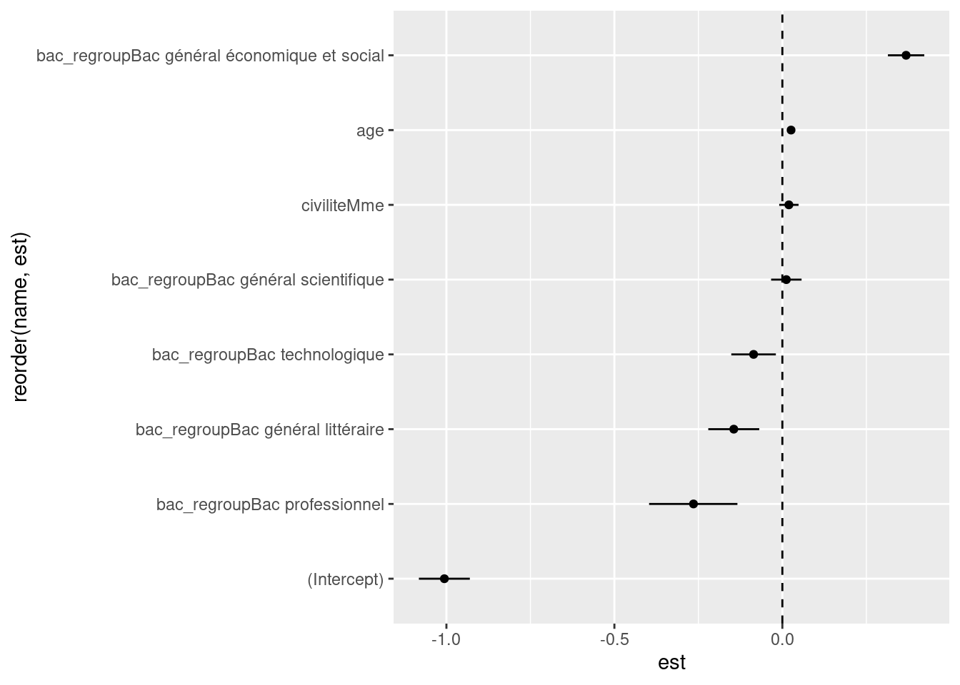
6.5 Les graines aléatoires
Un certain nombre de fonctions font appel à des générateurs aléatoires de nombres, ou des tirages aléatoires.
rnorm(5)[1] -2.4951748 -0.2541099 -1.2757394 -0.9043850 -0.0363517rnorm(5)[1] -0.2836808 1.4404653 -1.6611990 -1.6809537 1.0748188sample(1:10, 5)[1] 2 9 6 4 10sample(1:10, 5)[1] 6 3 4 10 2sample(1:6, 1)[1] 1sample(1:6, 1)[1] 4On peut étonnamment bloquer le générateur aléatoire pour sortir les mêmes valeurs lorsque l’on reproduit l’analyse (mais ces valeurs sont toujours aléatoires en soi !) :
set.seed(999)
rnorm(5)
[1] -0.2817402 -1.3125596 0.7951840 0.2700705 -0.2773064set.seed(999)
rnorm(5)[1] -0.2817402 -1.3125596 0.7951840 0.2700705 -0.2773064set.seed(42)
sample(1:10, 5)[1] 1 5 10 8 2set.seed(42)
sample(1:10, 5)[1] 1 5 10 8 26.6 Nuages de mots
Le traitement de texte (notamment la fouille de texte, en anglais text mining)
est un travail complexe, que ce soit sous R ou non. R fournit toutefois une
large palette d’outils, nativement ou bien dans des packages. Je renvois
notamment pour cela sur les packages tidytext, tm et textstem.
Une des applications concrètes est de faire un nuage de mots. Amusons-nous un
peu ici avec le package ggwordcloud qui permet de faire des nuages de mots
avancés dans le contexte de ggplot2 :
library("ggwordcloud")love_words# A tibble: 147 x 4
lang word native_speakers speakers
<chr> <chr> <dbl> <dbl>
1 zh 愛 1200 1200
2 en Love 400 800
3 es Amor 480 555
4 ar حب 245 515
5 hi प्यार 322 442
6 fr Amour 76.8 351.
7 bn ভালোবাসা 260 280
8 ms Cinta 77 277
9 pt Amor 220 243
10 ru Любовь 154 239
# … with 137 more rowssummary(love_words) lang word native_speakers speakers
Length:147 Length:147 Min. : 0.00 Min. : 0.00
Class :character Class :character 1st Qu.: 1.15 1st Qu.: 1.35
Mode :character Mode :character Median : 6.70 Median : 8.00
Mean : 41.03 Mean : 54.67
3rd Qu.: 34.00 3rd Qu.: 46.40
Max. :1200.00 Max. :1200.00 ggplot(love_words, aes(label = word)) +
geom_text_wordcloud() +
theme_minimal()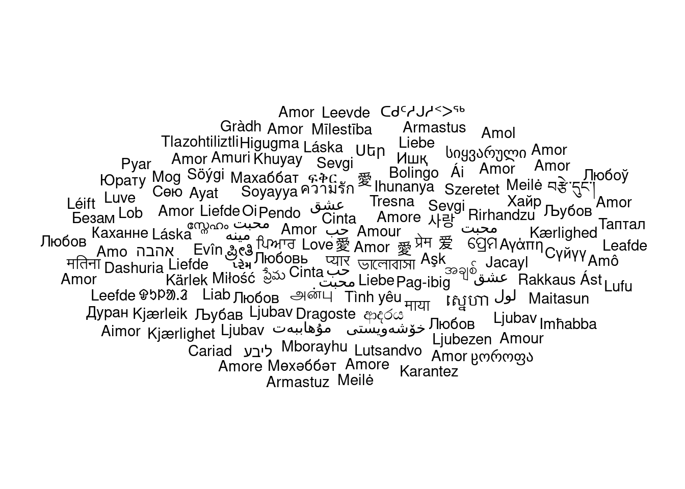
ggplot(love_words, aes(label = word, size = speakers)) +
  geom_text_wordcloud() +
  theme_minimal()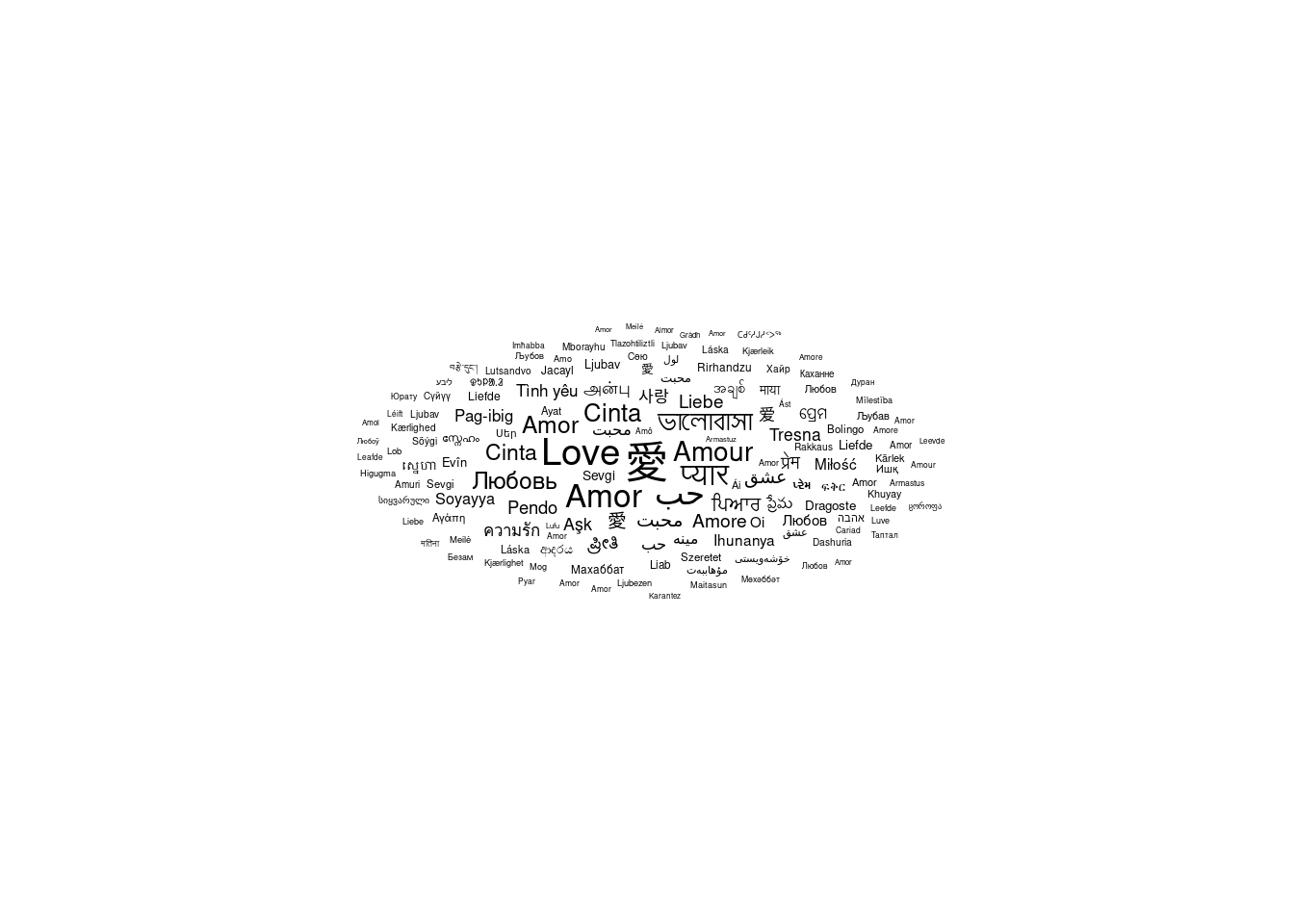
love_words %>%
  filter(speakers > 50) %>%
ggplot(aes(label = word, size = speakers)) +
  geom_text_wordcloud() +
  scale_size_area(max_size = 20) +
  theme_minimal()
set.seed(42)
love_words %>%
  filter(speakers > 50) %>%
ggplot(aes(label = word, size = speakers)) +
  geom_text_wordcloud() +
  scale_size_area(max_size = 20) +
  theme_minimal()
library("viridis")Loading required package: viridisLiteset.seed(42)
love_words %>%
filter(speakers > 50) %>%
ggplot(aes(label = word, size = speakers, color = speakers)) +
geom_text_wordcloud() +
scale_size_area(max_size = 20) +
scale_color_viridis(option = "plasma", end = .8, direction = -1) +
theme_minimal()
set.seed(42)
love_words %>%
  filter(speakers > 50) %>%
ggplot(aes(label = word, size = speakers, color = speakers)) +
  geom_text_wordcloud(eccentricity = 2) +
  scale_size_area(max_size = 20) +
  scale_color_viridis(option = "plasma", end = .8, direction = -1) +
  theme_minimal()
set.seed(42)
love_words %>%
  filter(speakers > 50) %>%
ggplot(aes(label = word, size = speakers, color = speakers)) +
  geom_text_wordcloud(eccentricity = 2, shape = "square") +
  scale_size_area(max_size = 20) +
  scale_color_viridis(option = "plasma", end = .8, direction = -1) +
  theme_minimal()
Dernier exemple, qui ne marche pas à tous les coups :
set.seed(42)
love_words %>%
  filter(speakers > 50) %>%
ggplot(aes(label = word, size = speakers, color = speakers)) +
  geom_text_wordcloud_area(
    mask = png::readPNG(system.file("extdata/hearth.png",
                                    package = "ggwordcloud", mustWork = TRUE
    )),
    rm_outside = TRUE
  ) +
  scale_size_area(max_size = 30) +
  scale_color_viridis(option = "plasma", end = .8, direction = -1) +
  theme_minimal()
6.7 Rapports paramétrés (parameterized reports)
rmarkdown::render("rapports/template-pdf.Rmd")
rmarkdown::render("rapports/template-pdf.Rmd", params = list(species = "setosa"))
rmarkdown::render("rapports/template-pdf.Rmd", params = list(species = "versicolor"))
for (i in unique(iris$Species))
rmarkdown::render("rapports/template-pdf.Rmd",
output_file = paste0(i, ".pdf"),
params = list(species = i)
)