29 Platanus hispanica
29.1 Données d’occurrences GBIF
Collecte des données du GBIF :
<<gbif download metadata>>
  Status: SUCCEEDED
  DOI: 10.15468/dl.tr8zzp
  Format: SIMPLE_CSV
  Download key: 0232026-230224095556074
  Created: 2023-05-11T06:36:46.402+00:00
  Modified: 2023-05-11T06:42:16.400+00:00
  Download link: https://api.gbif.org/v1/occurrence/download/request/0232026-230224095556074.zip
  Total records: 264214
Conversion en objets géographiques (format Simple feature de sf) et
exploration rapide des données (classe du jeu de données et premières lignes du
tableau) :
Simple feature collection with 7216 features and 50 fields
Attribute-geometry relationship: 50 constant, 0 aggregate, 0 identity
Geometry type: POINT
Dimension:     XY
Bounding box:  xmin: -123.169868 ymin: -44.417713 xmax: 175.055841 ymax: 59.34687
Geodetic CRS:  WGS 84
# A tibble: 7,216 × 51
    gbifID datasetKey occurrenceID kingdom phylum class order family genus species infraspecificEpithet
 * <int64> <chr>      <chr>        <chr>   <chr>  <chr> <chr> <chr>  <chr> <chr>   <chr>
 1    3.e9 5f06e39d-… USFS - New … Plantae Trach… Magn… Prot… Plata… Plat… Platan… ""
 2    3.e9 5f06e39d-… USFS - New … Plantae Trach… Magn… Prot… Plata… Plat… Platan… ""
 3    3.e9 d1e9202b-… NYCstreetTr… Plantae Trach… Magn… Prot… Plata… Plat… Platan… ""
 4    3.e9 c4e1739b-… BISON:New Y… Plantae Trach… Magn… Prot… Plata… Plat… Platan… ""
 5    3.e9 d1e9202b-… NYCstreetTr… Plantae Trach… Magn… Prot… Plata… Plat… Platan… ""
 6    3.e9 c4e1739b-… BISON:New Y… Plantae Trach… Magn… Prot… Plata… Plat… Platan… ""
 7    3.e9 c4e1739b-… BISON:New Y… Plantae Trach… Magn… Prot… Plata… Plat… Platan… ""
 8    3.e9 d1e9202b-… NYCstreetTr… Plantae Trach… Magn… Prot… Plata… Plat… Platan… ""
 9    3.e9 5f06e39d-… USFS - New … Plantae Trach… Magn… Prot… Plata… Plat… Platan… ""
10    3.e9 c4e1739b-… BISON:New Y… Plantae Trach… Magn… Prot… Plata… Plat… Platan… ""
# ℹ 7,206 more rows
# ℹ 40 more variables: taxonRank <chr>, scientificName <chr>, verbatimScientificName <chr>,
#   verbatimScientificNameAuthorship <chr>, countryCode <chr>, locality <chr>, stateProvince <chr>,
#   occurrenceStatus <chr>, individualCount <int>, publishingOrgKey <chr>, decimalLatitude <dbl>,
#   decimalLongitude <dbl>, coordinateUncertaintyInMeters <dbl>, coordinatePrecision <dbl>,
#   elevation <dbl>, elevationAccuracy <dbl>, depth <dbl>, depthAccuracy <dbl>, eventDate <dttm>,
#   day <int>, month <int>, year <int>, taxonKey <int>, speciesKey <int>, basisOfRecord <chr>, …
Il y a 7 216 occurrences dans le jeu de données. On les affiche sur la carte du monde :
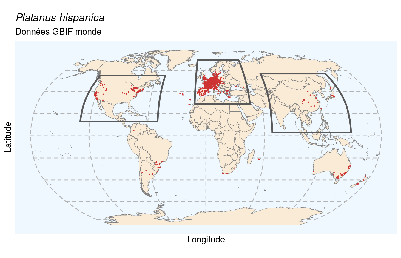
Figure 29.1: Occurrences de Platanus hispanica dans le monde.
29.1.1 Données par région
On évalue la proportion d’occurrences dans chaque région, en utilisant les 3 masques créés précédemment. Si on a au moins 50 % des occurrences dans une région, on peut continuer en travaillant uniquement sur ces données. Sinon, on vérifie qu’au moins 67 % des données tombent dans l’ensemble des régions, et on prend la région la plus représentée. Au final, s’il s’agit d’une espèce endémique d’Europe, on n’a pas besoin de manipulation supplémentaire.
[1] 0.9131097561[1] 0.05349223947[1] 0.004988913525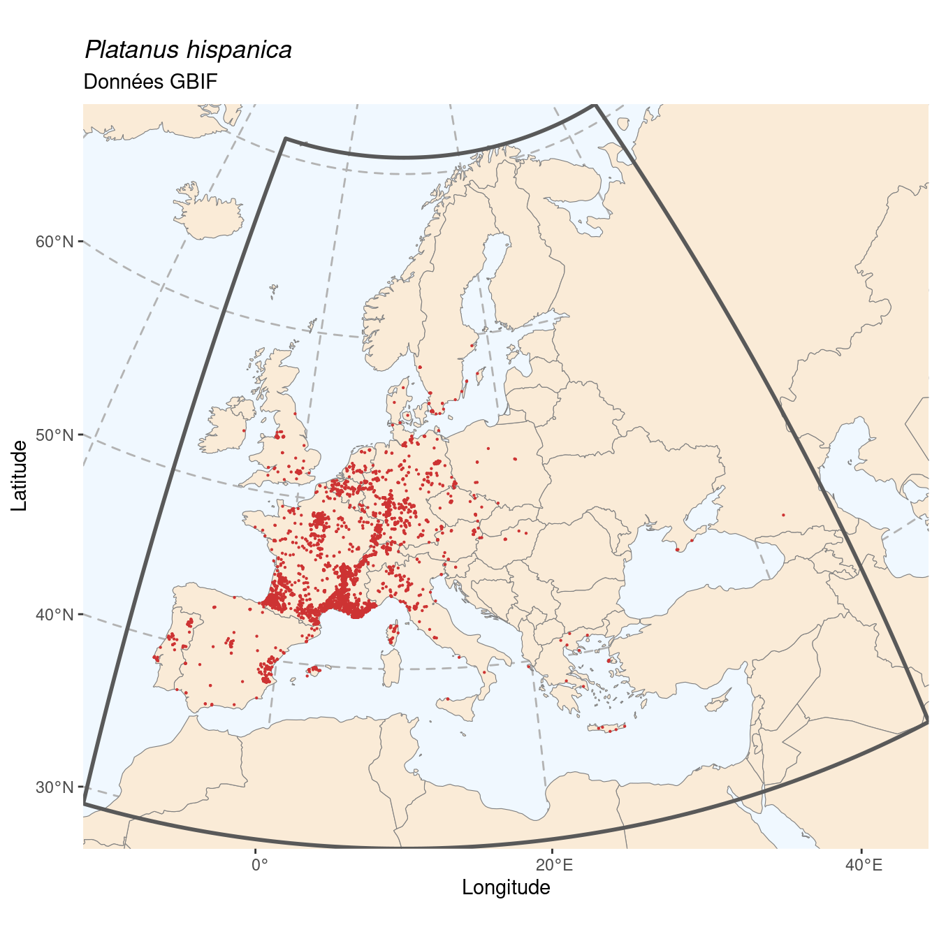
Figure 29.2: Occurrence de Platanus hispanica dans la région d’endémisme.
29.1.2 Licences
On s’intéresse ici au problème particulier des licences :
   CC_BY_4_0 CC_BY_NC_4_0      CC0_1_0
        5302         1056          231
[1] 83.97328881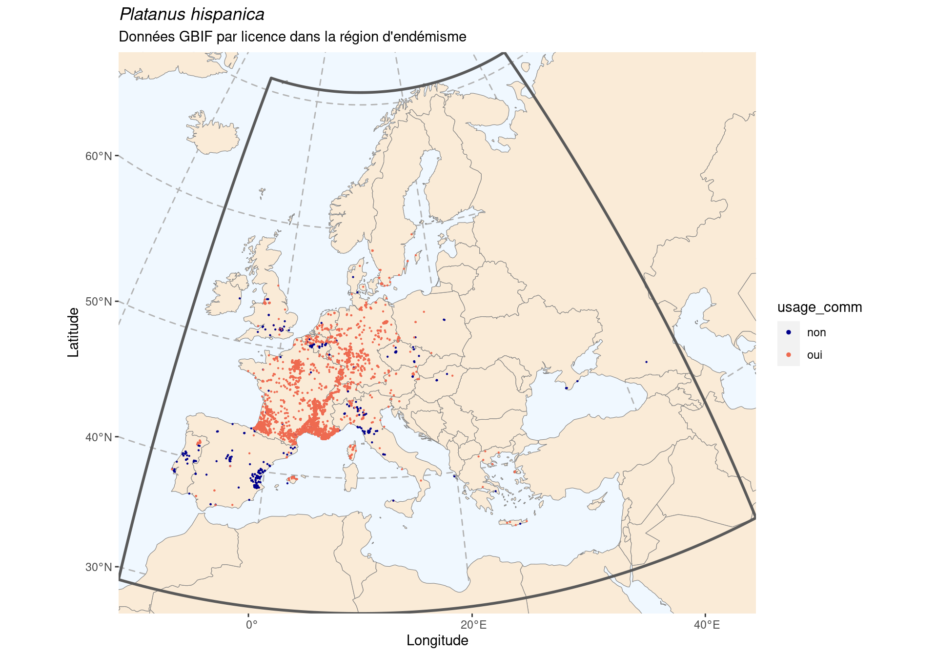
Figure 29.3: Occurrence de Platanus hispanica dans la région d’endémisme, selon la licence : CC BY-NC en bleu ; CC0 et CC BY en orange.
Idéalement, on aimerait avoir au moins 50 % de données vraiment libres
d’utilisation (c’est-à-dire sans la clause -NC). On continue en supprimant les
données en CC BY-NC.
[1] 553329.1.3 Sous-échantillonnage
Si le jeu de données contient 25 000 occurrences ou plus, on procède au sous-échantillonnage aléatoire pour en conserver un maximum de 25 000.
Simple feature collection with 5533 features and 50 fields
Attribute-geometry relationship: 50 constant, 0 aggregate, 0 identity
Geometry type: POINT
Dimension:     XY
Bounding box:  xmin: -9.429703 ymin: 34.9729 xmax: 26.244364 ymax: 59.34687
Geodetic CRS:  WGS 84
# A tibble: 5,533 × 51
    gbifID datasetKey occurrenceID kingdom phylum class order family genus species infraspecificEpithet
   <int64> <chr>      <chr>        <chr>   <chr>  <chr> <chr> <chr>  <chr> <chr>   <chr>
 1     1e9 75956ee6-… http://cbnm… Plantae Trach… Magn… Prot… Plata… Plat… Platan… ""
 2     1e9 75956ee6-… http://pifh… Plantae Trach… Magn… Prot… Plata… Plat… Platan… ""
 3     1e9 75956ee6-… http://flor… Plantae Trach… Magn… Prot… Plata… Plat… Platan… ""
 4     1e9 75956ee6-… http://flor… Plantae Trach… Magn… Prot… Plata… Plat… Platan… ""
 5     1e9 75956ee6-… http://pifh… Plantae Trach… Magn… Prot… Plata… Plat… Platan… ""
 6     1e9 75956ee6-… http://flor… Plantae Trach… Magn… Prot… Plata… Plat… Platan… ""
 7     1e9 75956ee6-… http://pifh… Plantae Trach… Magn… Prot… Plata… Plat… Platan… ""
 8     1e9 75956ee6-… http://ofsa… Plantae Trach… Magn… Prot… Plata… Plat… Platan… ""
 9     1e9 75956ee6-… http://flor… Plantae Trach… Magn… Prot… Plata… Plat… Platan… ""
10     1e9 75956ee6-… http://flor… Plantae Trach… Magn… Prot… Plata… Plat… Platan… ""
# ℹ 5,523 more rows
# ℹ 40 more variables: taxonRank <chr>, scientificName <chr>, verbatimScientificName <chr>,
#   verbatimScientificNameAuthorship <chr>, countryCode <chr>, locality <chr>, stateProvince <chr>,
#   occurrenceStatus <chr>, individualCount <int>, publishingOrgKey <chr>, decimalLatitude <dbl>,
#   decimalLongitude <dbl>, coordinateUncertaintyInMeters <dbl>, coordinatePrecision <dbl>,
#   elevation <dbl>, elevationAccuracy <dbl>, depth <dbl>, depthAccuracy <dbl>, eventDate <dttm>,
#   day <int>, month <int>, year <int>, taxonKey <int>, speciesKey <int>, basisOfRecord <chr>, …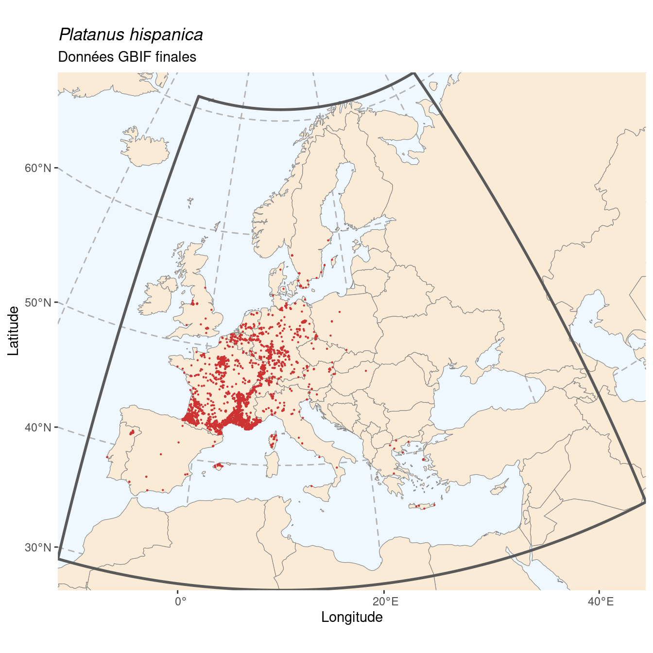
29.2 Modélisation de la niche climatique
29.2.1 Préparer les données
Organisation des données d’entrées (occurrences et données environnementales) et des données produites de pseudo-absences :
 class       : SpatVector
 geometry    : points
 dimensions  : 5533, 0  (geometries, attributes)
 extent      : -9.429703, 26.24436, 34.9729, 59.34687  (xmin, xmax, ymin, ymax)
 coord. ref. : lon/lat WGS 84 (EPSG:4326)
-=-=-=-=-=-=-=-=-=-=-=-=-=-=-= plhi Data Formating -=-=-=-=-=-=-=-=-=-=-=-=-=-=-=

      ! Response variable is considered as only presences... Is it really what you want?
      ! No data has been set aside for modeling evaluation
 !!! Some data are located in the same raster cell.
          Please set `filter.raster = TRUE` if you want an automatic filtering.

Checking Pseudo-absence selection arguments...

   > random pseudo absences selection
   > Pseudo absences are selected in explanatory variables
 ! Some NAs have been automatically removed from your data
 !!! Some data are located in the same raster cell.
          Please set `filter.raster = TRUE` if you want an automatic filtering.
-=-=-=-=-=-=-=-=-=-=-=-=-=-=-=-=-=-= Done -=-=-=-=-=-=-=-=-=-=-=-=-=-=-=-=-=-=
-=-=-=-=-=-=-=-=-=-=-=-=-=-= BIOMOD.formated.data -=-=-=-=-=-=-=-=-=-=-=-=-=-=

dir.name =  Output

sp.name =  plhi

     5519 presences,  0 true absences and  16505 undefined points in dataset


     6 explanatory variables

 temp_max_august    temp_min       temp_wet_quart     temp_season
 Min.   : 0.50   Min.   :-21.768   Min.   :-11.467   Min.   :   0.0
 1st Qu.:20.93   1st Qu.: -8.697   1st Qu.:  9.764   1st Qu.: 615.6
 Median :24.95   Median : -1.776   Median : 13.176   Median : 716.5
 Mean   :25.51   Mean   : -3.592   Mean   : 12.663   Mean   : 752.1
 3rd Qu.:28.69   3rd Qu.:  1.696   3rd Qu.: 16.320   3rd Qu.: 894.9
 Max.   :44.88   Max.   : 10.589   Max.   : 24.703   Max.   :1373.9
 prec_wet_quart    prec_season
 Min.   :   5.0   Min.   :  7.483
 1st Qu.: 176.0   1st Qu.: 23.066
 Median : 220.0   Median : 31.850
 Mean   : 223.2   Mean   : 35.867
 3rd Qu.: 264.0   3rd Qu.: 40.589
 Max.   :1222.0   Max.   :123.444

-=-=-=-=-=-=-=-=-=-=-=-=-=-=-=-=-=-=-=-=-=-=-=-=-=-=-=-=-=-=-=-=-=-=-=-=-=-=-=-=
On visualise les pseudo-absences :
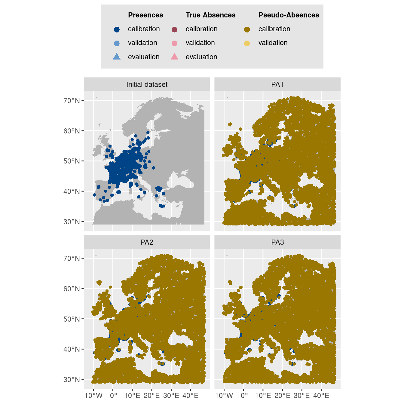
Figure 29.5: Les données d’occurrences (en haut à gauche) et les trois jeux de données aléatoires de pseudo-absences.
$data.vect
 class       : SpatVector
 geometry    : points
 dimensions  : 38675, 2  (geometries, attributes)
 extent      : -10.39583, 46.97917, 29.02083, 70.97917  (xmin, xmax, ymin, ymax)
 coord. ref. :
 names       :  resp         dataset
 type        : <num>           <chr>
 values      :    10 Initial dataset
                  10 Initial dataset
                  10 Initial dataset

$data.label
                              9                              10
                "**Presences**"       "Presences (calibration)"
                             11                              12
       "Presences (validation)"        "Presences (evaluation)"
                             19                              20
            "**True Absences**"   "True Absences (calibration)"
                             21                              22
   "True Absences (validation)"    "True Absences (evaluation)"
                             29                              30
          "**Pseudo-Absences**" "Pseudo-Absences (calibration)"
                             31                               1
 "Pseudo-Absences (validation)"                    "Background"

$data.plot
Figure 29.6: Les données d’occurrences (en haut à gauche) et les trois jeux de données aléatoires de pseudo-absences.
29.2.2 Modèles individuels de niche
-=-=-=-=-=-=-=-=-=-=-=-=-=-=-= Build Single Models -=-=-=-=-=-=-=-=-=-=-=-=-=-=-=


Checking Models arguments...

Creating suitable Workdir...

            ! Weights where automatically defined for plhi_PA1 to rise a 0.5 prevalence !
            ! Weights where automatically defined for plhi_PA2 to rise a 0.5 prevalence !
            ! Weights where automatically defined for plhi_PA3 to rise a 0.5 prevalence !


-=-=-=-=-=-=-=-=-=-=-=-=-=-= plhi Modeling Summary -=-=-=-=-=-=-=-=-=-=-=-=-=-=

 6  environmental variables ( temp_max_august temp_min temp_wet_quart temp_season prec_wet_quart prec_season )
Number of evaluation repetitions : 1
Models selected : GAM MARS MAXNET GBM ANN RF

Total number of model runs: 18

-=-=-=-=-=-=-=-=-=-=-=-=-=-=-=-=-=-=-=-=-=-=-=-=-=-=-=-=-=-=-=-=-=-=-=-=-=-=-=-=


-=-=-=- Run :  plhi_PA1


-=-=-=--=-=-=- plhi_PA1_RUN1


-=-=-=- Run :  plhi_PA2


-=-=-=--=-=-=- plhi_PA2_RUN1


-=-=-=- Run :  plhi_PA3


-=-=-=--=-=-=- plhi_PA3_RUN1

-=-=-=-=-=-=-=-=-=-=-=-=-=-=-=-=-=-= Done -=-=-=-=-=-=-=-=-=-=-=-=-=-=-=-=-=-=
29.2.2.1 Évaluation de la performance
             full.name  PA  run   algo metric.eval cutoff sensitivity
1    plhi_PA1_RUN1_GAM PA1 RUN1    GAM         TSS  444.0      98.075
2    plhi_PA1_RUN1_GAM PA1 RUN1    GAM         ROC  509.5      97.441
3   plhi_PA1_RUN1_MARS PA1 RUN1   MARS         TSS  463.0      96.557
4   plhi_PA1_RUN1_MARS PA1 RUN1   MARS         ROC  454.5      96.716
5 plhi_PA1_RUN1_MAXNET PA1 RUN1 MAXNET         TSS  348.0      96.285
6 plhi_PA1_RUN1_MAXNET PA1 RUN1 MAXNET         ROC  358.5      95.810
  specificity calibration validation evaluation
1      60.235       0.583      0.591         NA
2      60.935       0.731      0.730         NA
3      87.912       0.845      0.842         NA
4      87.822       0.964      0.960         NA
5      88.771       0.851      0.839         NA
6      89.404       0.966      0.963         NA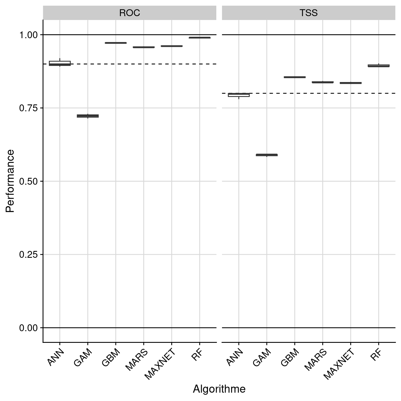
Figure 29.7: Évaluation de la performance des modèles individuels : True Skill Statistic & aire sous la courbe de ROC.
29.2.2.2 Importance des variables environnementales
          full.name  PA  run algo        expl.var rand  var.imp
1 plhi_PA1_RUN1_GAM PA1 RUN1  GAM temp_max_august    1 0.103510
2 plhi_PA1_RUN1_GAM PA1 RUN1  GAM        temp_min    1 0.380937
3 plhi_PA1_RUN1_GAM PA1 RUN1  GAM  temp_wet_quart    1 0.015113
4 plhi_PA1_RUN1_GAM PA1 RUN1  GAM     temp_season    1 0.247897
5 plhi_PA1_RUN1_GAM PA1 RUN1  GAM  prec_wet_quart    1 0.011113
6 plhi_PA1_RUN1_GAM PA1 RUN1  GAM     prec_season    1 0.052348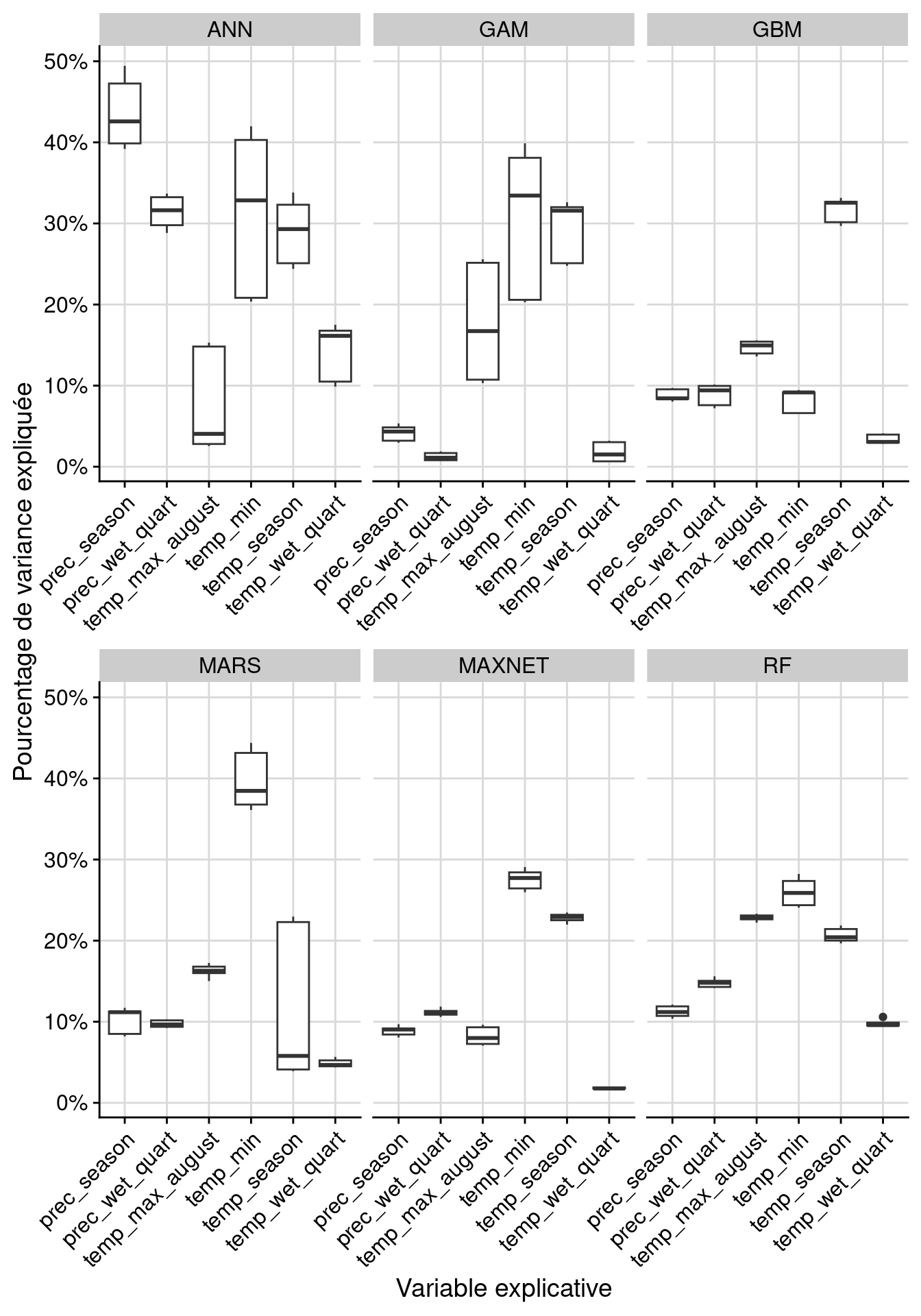
Figure 29.8: Pourcentage de variance expliquée pour chaque variable, décomposé par algorithme.
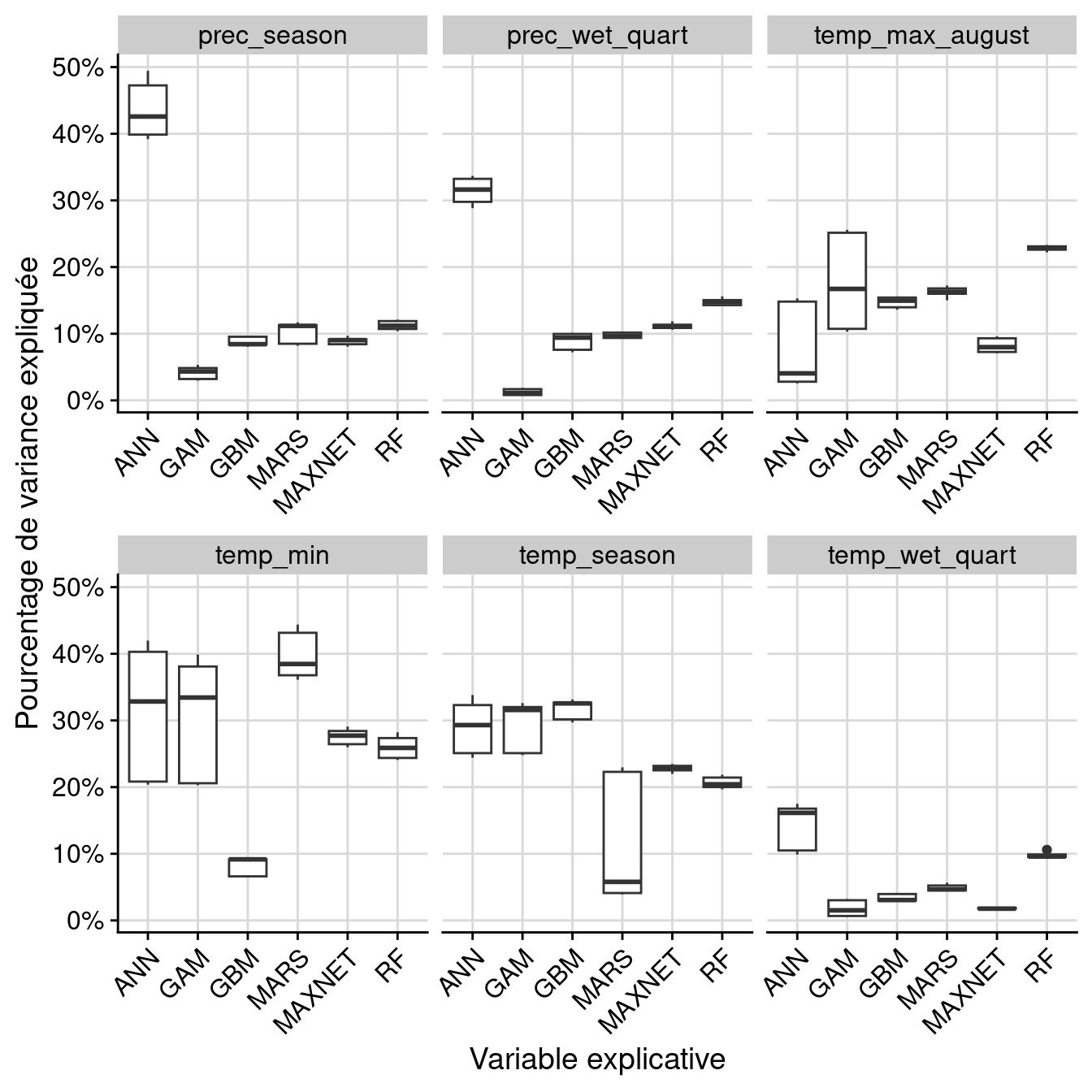
Figure 29.9: Pourcentage de variance expliquée pour chaque variable, décomposé par variable.
29.2.3 Modèles d’ensemble de niche
Seulement modèles avec TSS > 0.8
-=-=-=-=-=-=-=-=-=-=-=-=-= BIOMOD.ensemble.models.out -=-=-=-=-=-=-=-=-=-=-=-=-=

sp.name : plhi

expl.var.names : temp_max_august temp_min temp_wet_quart temp_season
prec_wet_quart prec_season


models computed:
plhi_EMcvByTSS_mergedData_mergedRun_mergedAlgo, plhi_EMwmeanByTSS_mergedData_mergedRun_mergedAlgo

models failed: none

-=-=-=-=-=-=-=-=-=-=-=-=-=-=-=-=-=-=-=-=-=-=-=-=-=-=-=-=-=-=-=-=-=-=-=-=-=-=-=-=
29.2.3.1 Évaluation de la qualité
                                          full.name merged.by.PA merged.by.run
1 plhi_EMwmeanByTSS_mergedData_mergedRun_mergedAlgo   mergedData     mergedRun
2 plhi_EMwmeanByTSS_mergedData_mergedRun_mergedAlgo   mergedData     mergedRun
  merged.by.algo filtered.by    algo metric.eval cutoff sensitivity specificity
1     mergedAlgo         TSS EMwmean         TSS  604.0      94.709      94.311
2     mergedAlgo         TSS EMwmean         ROC  645.5      93.858      95.304
  calibration validation evaluation
1       0.891         NA         NA
2       0.990         NA         NA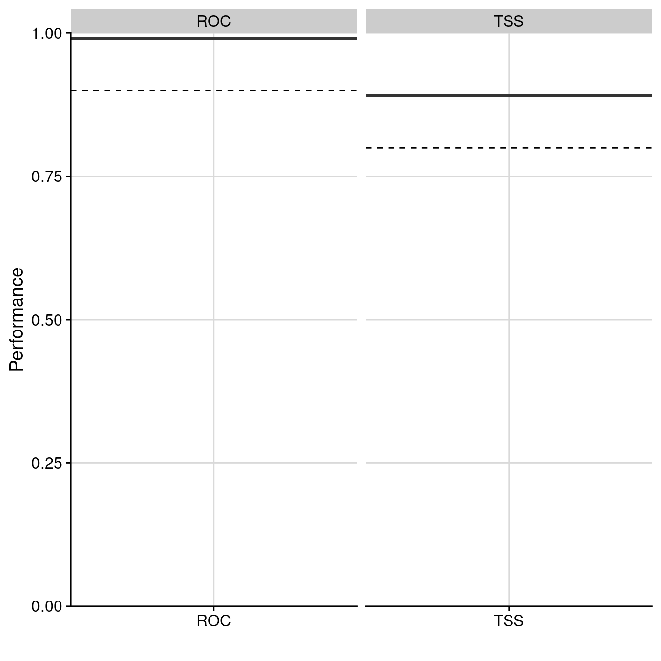
Figure 29.11: Évaluation de la qualité du modèle d’ensemble : Aire sous la courbe de ROC & True Skill Statistic.
                                       full.name merged.by.PA merged.by.run
1 plhi_EMcvByTSS_mergedData_mergedRun_mergedAlgo   mergedData     mergedRun
2 plhi_EMcvByTSS_mergedData_mergedRun_mergedAlgo   mergedData     mergedRun
3 plhi_EMcvByTSS_mergedData_mergedRun_mergedAlgo   mergedData     mergedRun
4 plhi_EMcvByTSS_mergedData_mergedRun_mergedAlgo   mergedData     mergedRun
5 plhi_EMcvByTSS_mergedData_mergedRun_mergedAlgo   mergedData     mergedRun
6 plhi_EMcvByTSS_mergedData_mergedRun_mergedAlgo   mergedData     mergedRun
  merged.by.algo filtered.by algo        expl.var rand  var.imp
1     mergedAlgo         TSS EMcv temp_max_august    1 0.184667
2     mergedAlgo         TSS EMcv        temp_min    1 0.345774
3     mergedAlgo         TSS EMcv  temp_wet_quart    1 0.050990
4     mergedAlgo         TSS EMcv     temp_season    1 0.248789
5     mergedAlgo         TSS EMcv  prec_wet_quart    1 0.183716
6     mergedAlgo         TSS EMcv     prec_season    1 0.103680
Par variable :
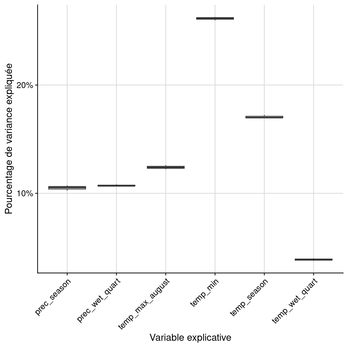
Figure 29.12: Pourcentage de variance expliquée par variable dans le modèle d’ensemble.
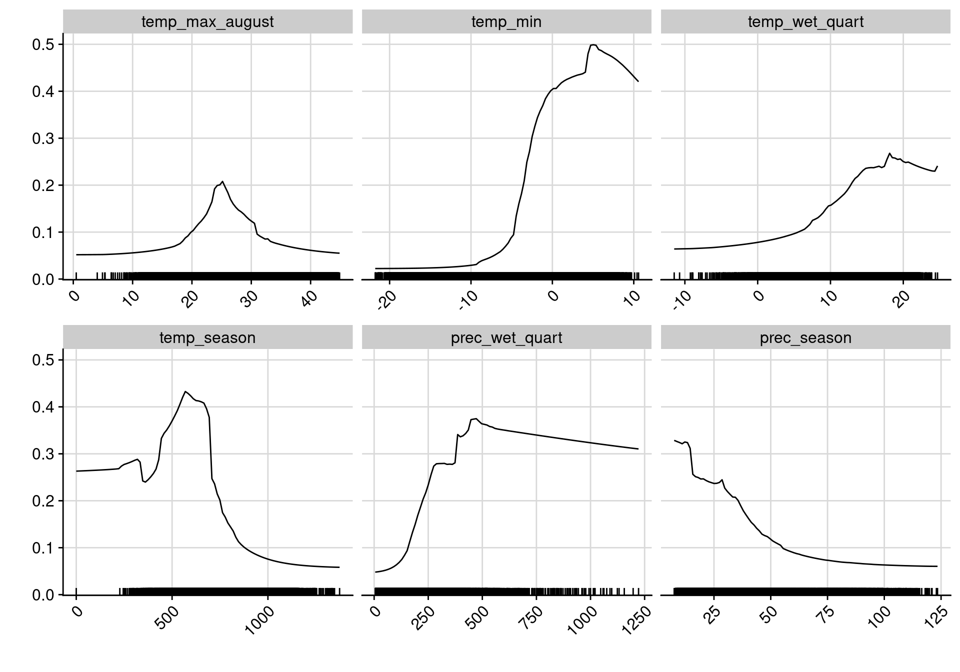
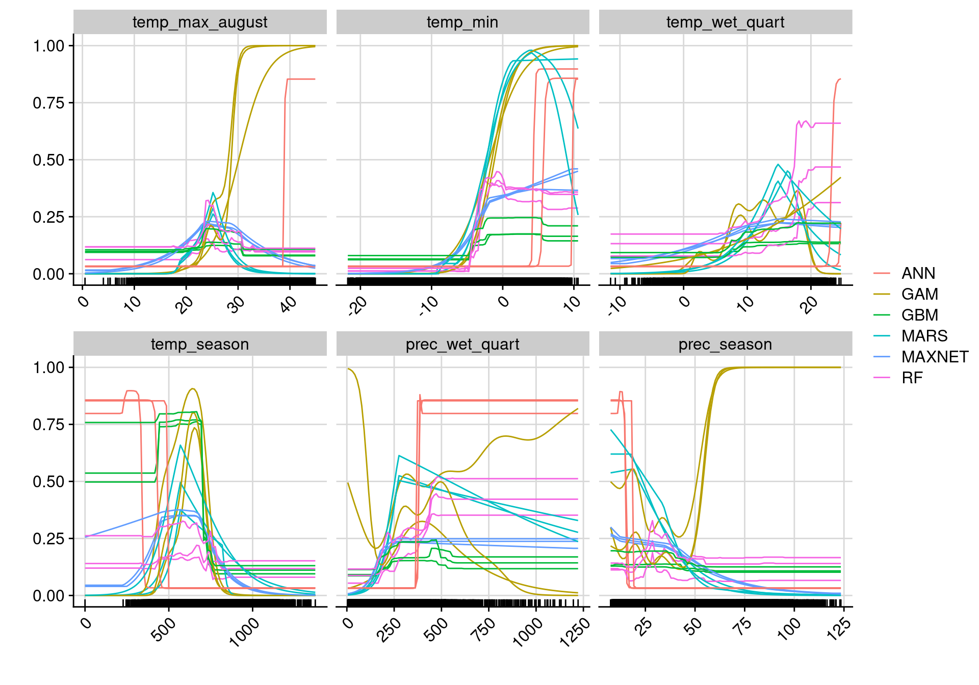
Figure 29.13: Courbes de réponse de chaque variable climatique dans le modèle d’ensemble.
29.3 Projections
29.3.1 Distribution potentielle contemporaine
Contemporaine : Cartographie des observations sur couches climatiques Extraction des conditions climatiques favorables
-=-=-=-=-=-=-=-=-=-=-=-=-=-= BIOMOD.projection.out -=-=-=-=-=-=-=-=-=-=-=-=-=-=

Projection directory : Output/plhi/current


sp.name : plhi

expl.var.names : temp_max_august temp_min temp_wet_quart temp_season
prec_wet_quart prec_season


modeling.id : AllModels ( Output/plhi/plhi.AllModels.models.out )

models.projected :
plhi_PA1_RUN1_GAM, plhi_PA1_RUN1_MARS, plhi_PA1_RUN1_MAXNET, plhi_PA1_RUN1_GBM, plhi_PA1_RUN1_ANN, plhi_PA1_RUN1_RF, plhi_PA2_RUN1_GAM, plhi_PA2_RUN1_MARS, plhi_PA2_RUN1_MAXNET, plhi_PA2_RUN1_GBM, plhi_PA2_RUN1_ANN, plhi_PA2_RUN1_RF, plhi_PA3_RUN1_GAM, plhi_PA3_RUN1_MARS, plhi_PA3_RUN1_MAXNET, plhi_PA3_RUN1_GBM, plhi_PA3_RUN1_ANN, plhi_PA3_RUN1_RF

available binary projection : TSS, ROC

available filtered projection : TSS, ROC

-=-=-=-=-=-=-=-=-=-=-=-=-=-=-=-=-=-=-=-=-=-=-=-=-=-=-=-=-=-=-=-=-=-=-=-=-=-=-=-=
Figure 29.14: Projection de la distribution potentielle contemporaine sur l’Europe, selon les 6 algorithmes et les 3 runs.
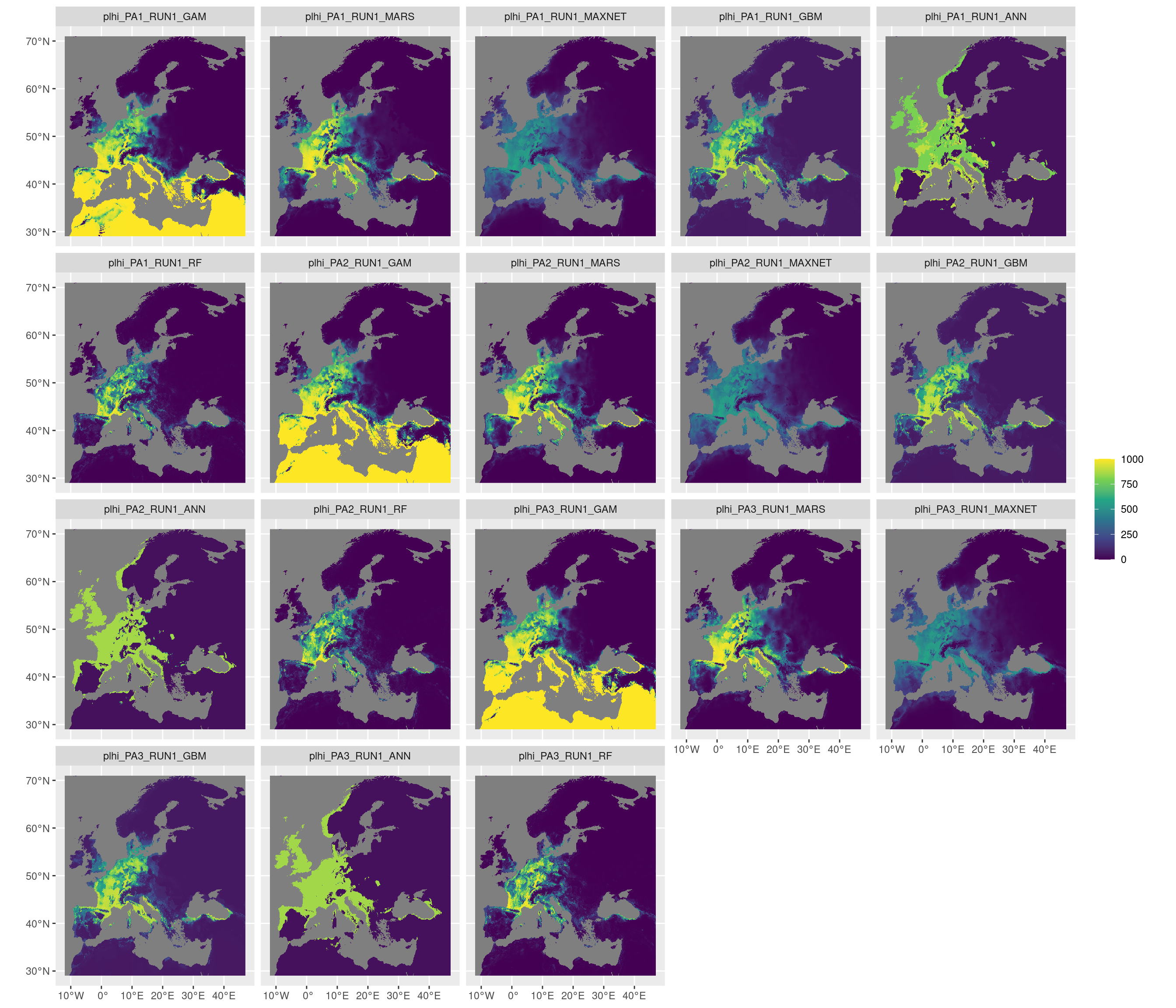
Figure 29.15: Projection de la distribution potentielle contemporaine sur l’Europe, selon les 6 algorithmes et les 3 runs.
-=-=-=-=-=-=-=-=-=-=-=-=-=-= BIOMOD.projection.out -=-=-=-=-=-=-=-=-=-=-=-=-=-=

Projection directory : Output/plhi/current


sp.name : plhi

expl.var.names : temp_max_august temp_min temp_wet_quart temp_season
prec_wet_quart prec_season


modeling.id : AllModels ( Output/plhi/plhi.AllModels.ensemble.models.out )

models.projected :
plhi_EMcvByTSS_mergedData_mergedRun_mergedAlgo, plhi_EMwmeanByTSS_mergedData_mergedRun_mergedAlgo

-=-=-=-=-=-=-=-=-=-=-=-=-=-=-=-=-=-=-=-=-=-=-=-=-=-=-=-=-=-=-=-=-=-=-=-=-=-=-=-=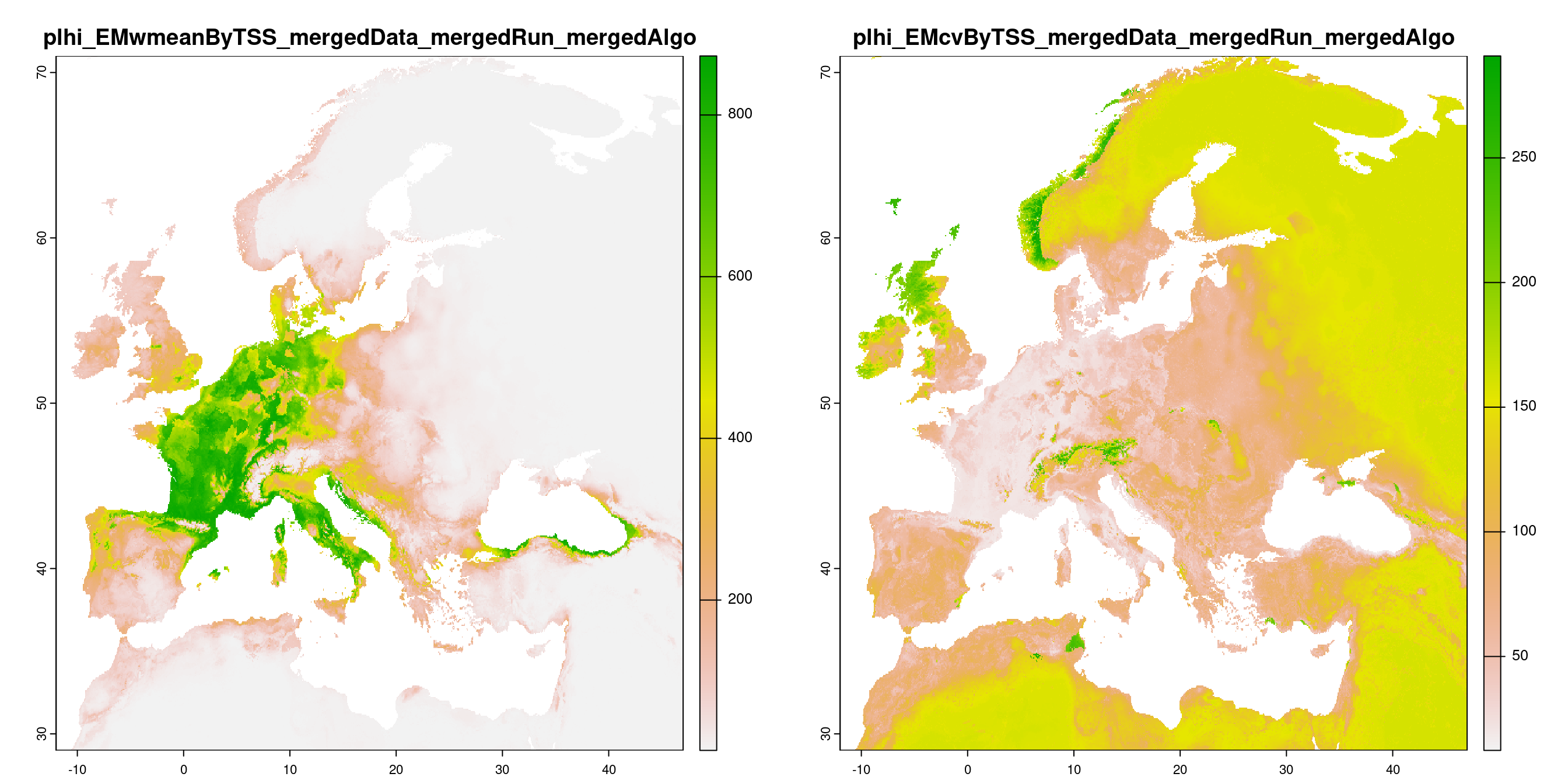
Figure 29.16: A) Projection de la distribution potentielle contemporaine (modèle d’ensemble) ; B) Incertitude associée à la projection.
29.3.2 Interpolation à l’échelle de la métropole
- → conditions climatiques favorables à fine échelle
On projette la niche climatique sur ce raster à fine échelle.
-=-=-=-=-=-=-=-=-=-=-=-=-=-= BIOMOD.projection.out -=-=-=-=-=-=-=-=-=-=-=-=-=-=

Projection directory : Output/plhi/cont_gre


sp.name : plhi

expl.var.names : temp_max_august temp_min temp_wet_quart temp_season
prec_wet_quart prec_season


modeling.id : AllModels ( Output/plhi/plhi.AllModels.models.out )

models.projected :
plhi_PA1_RUN1_GAM, plhi_PA1_RUN1_MARS, plhi_PA1_RUN1_MAXNET, plhi_PA1_RUN1_GBM, plhi_PA1_RUN1_ANN, plhi_PA1_RUN1_RF, plhi_PA2_RUN1_GAM, plhi_PA2_RUN1_MARS, plhi_PA2_RUN1_MAXNET, plhi_PA2_RUN1_GBM, plhi_PA2_RUN1_ANN, plhi_PA2_RUN1_RF, plhi_PA3_RUN1_GAM, plhi_PA3_RUN1_MARS, plhi_PA3_RUN1_MAXNET, plhi_PA3_RUN1_GBM, plhi_PA3_RUN1_ANN, plhi_PA3_RUN1_RF

available binary projection : TSS, ROC

available filtered projection : TSS, ROC

-=-=-=-=-=-=-=-=-=-=-=-=-=-=-=-=-=-=-=-=-=-=-=-=-=-=-=-=-=-=-=-=-=-=-=-=-=-=-=-=
Figure 29.17: Projection de la distribution potentielle contemporaine sur la métropole de Grenoble, selon les 6 algorithmes et les 3 runs.
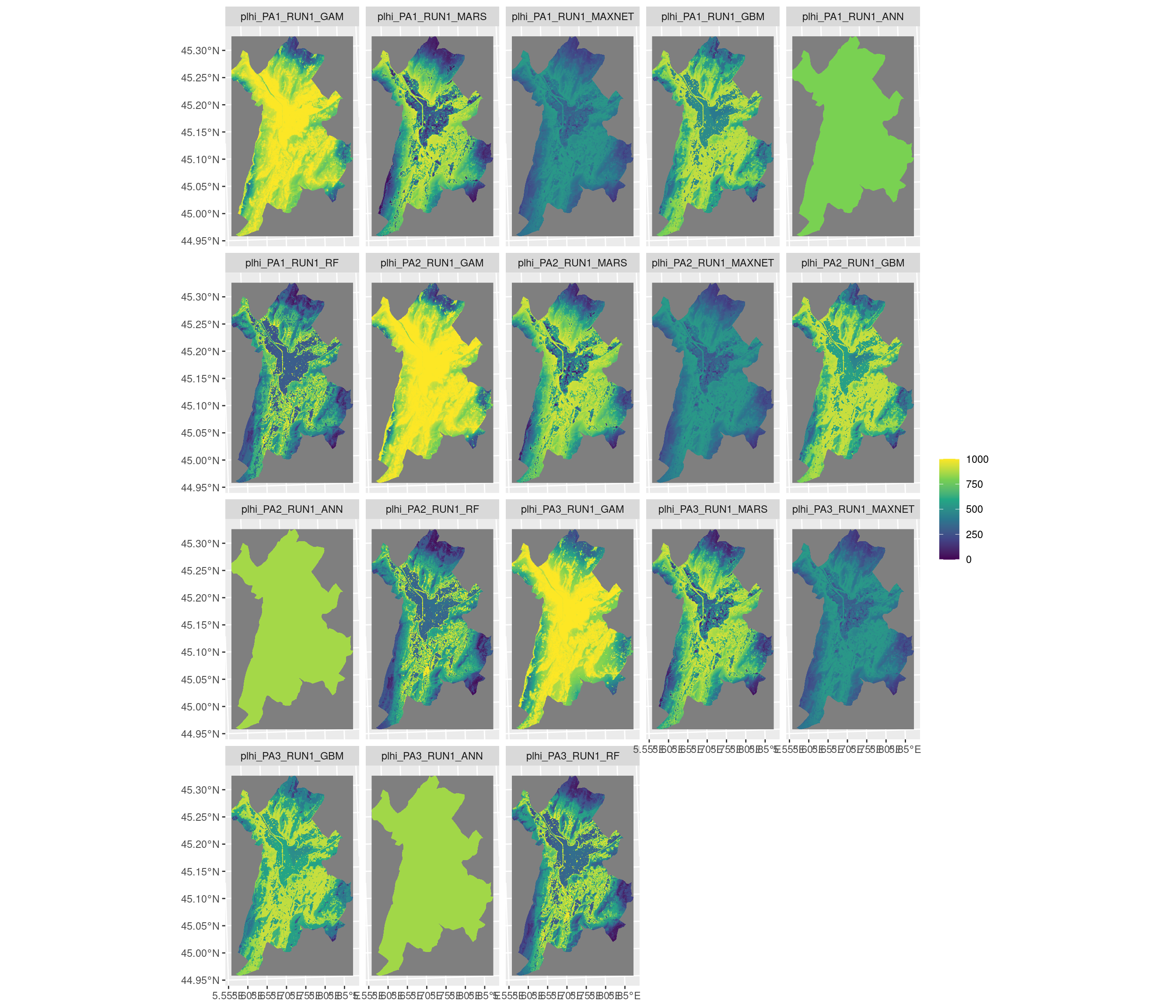
Figure 29.18: Projection de la distribution potentielle contemporaine sur la métropole de Grenoble, selon les 6 algorithmes et les 3 runs.
-=-=-=-=-=-=-=-=-=-=-=-=-=-= BIOMOD.projection.out -=-=-=-=-=-=-=-=-=-=-=-=-=-=

Projection directory : Output/plhi/cont_gre


sp.name : plhi

expl.var.names : temp_max_august temp_min temp_wet_quart temp_season
prec_wet_quart prec_season


modeling.id : AllModels ( Output/plhi/plhi.AllModels.ensemble.models.out )

models.projected :
plhi_EMcvByTSS_mergedData_mergedRun_mergedAlgo, plhi_EMwmeanByTSS_mergedData_mergedRun_mergedAlgo

-=-=-=-=-=-=-=-=-=-=-=-=-=-=-=-=-=-=-=-=-=-=-=-=-=-=-=-=-=-=-=-=-=-=-=-=-=-=-=-=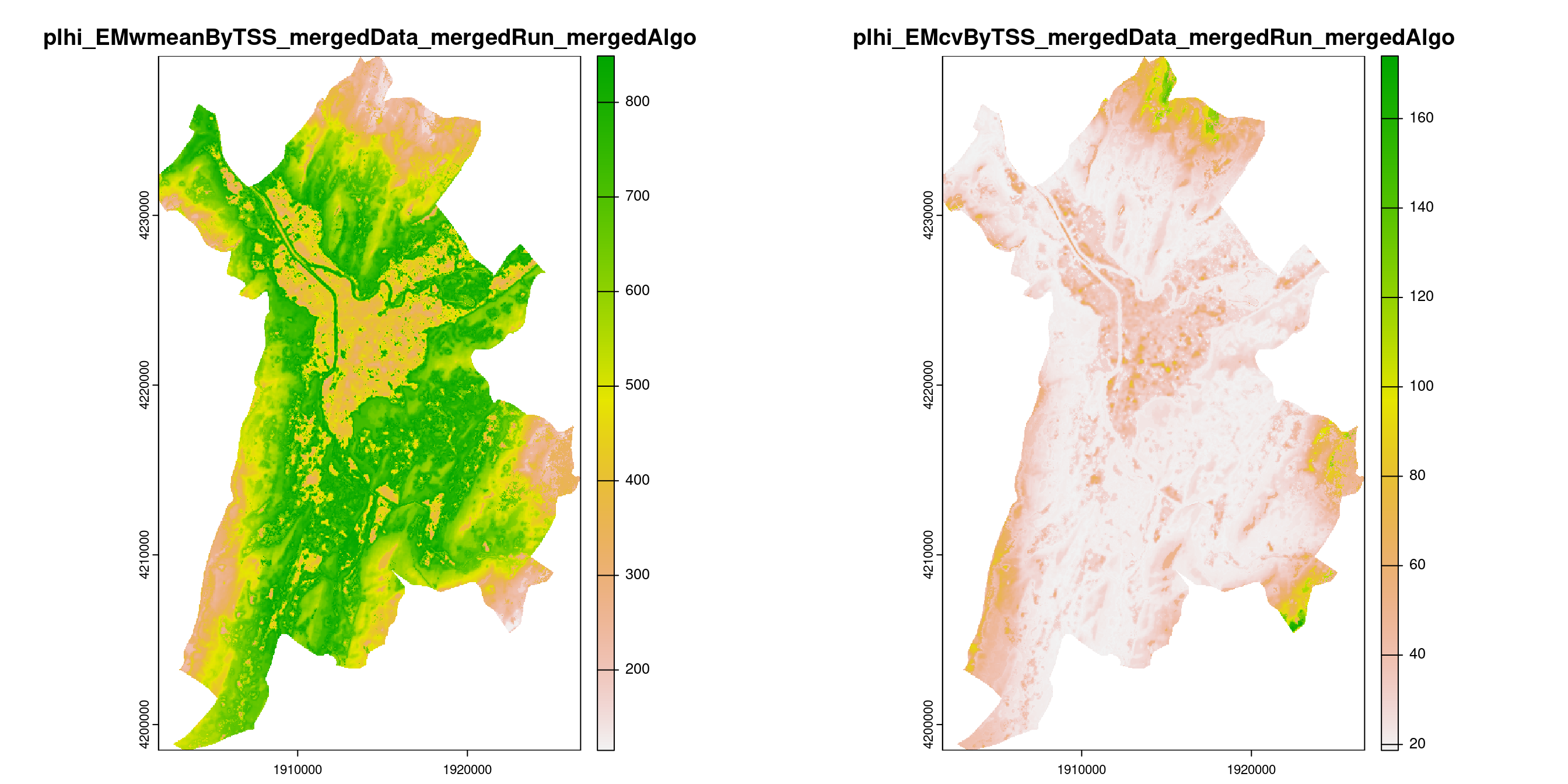
Figure 29.19: A) Projection de la distribution potentielle contemporaine (modèle d’ensemble) sur la métropole de Grenoble ; B) Incertitude associée à la projection.
29.3.3 Distributions potentielles futures
Futur : Projection à l’échelle de l’Europe jusqu’à l’horizon 2100
Toutes les fenêtres temporelles × scénarios pour le GCM « IPSL-CM6A-LR »
- SSP1-2.6

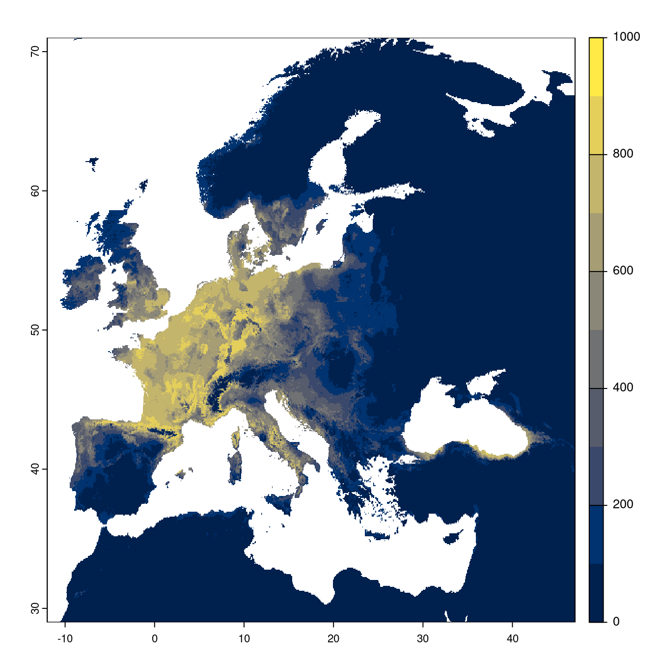

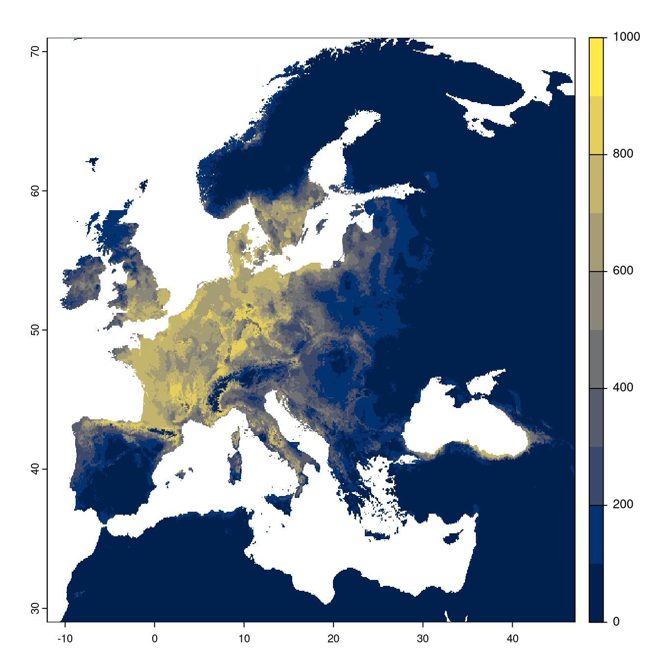

Figure 29.20: Projection des distributions potentielles futures jusqu’à l’horizon 2100 sous le scénario SSP1-2.6 (modèle d’ensemble).
On obtient pour la métrique TSS une carte unique de moyenne pondérée sur les algorithmes et sur les jeux de pseudo-absences.
- SSP2-4.5
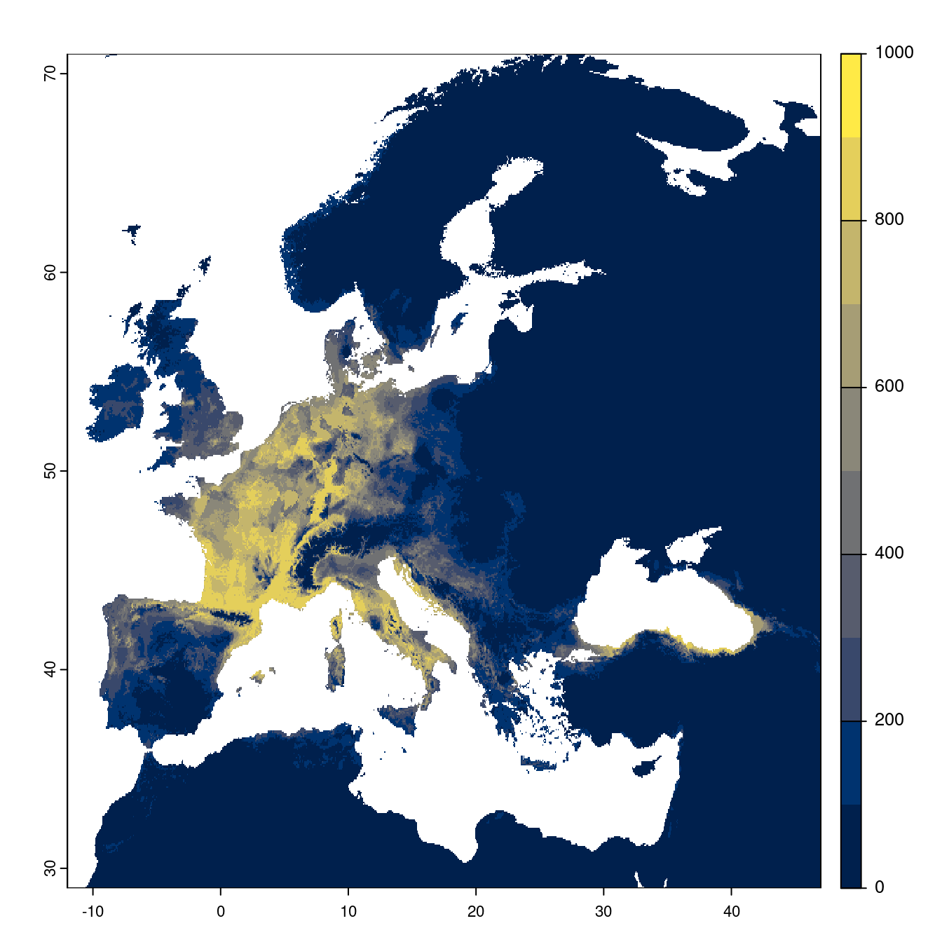
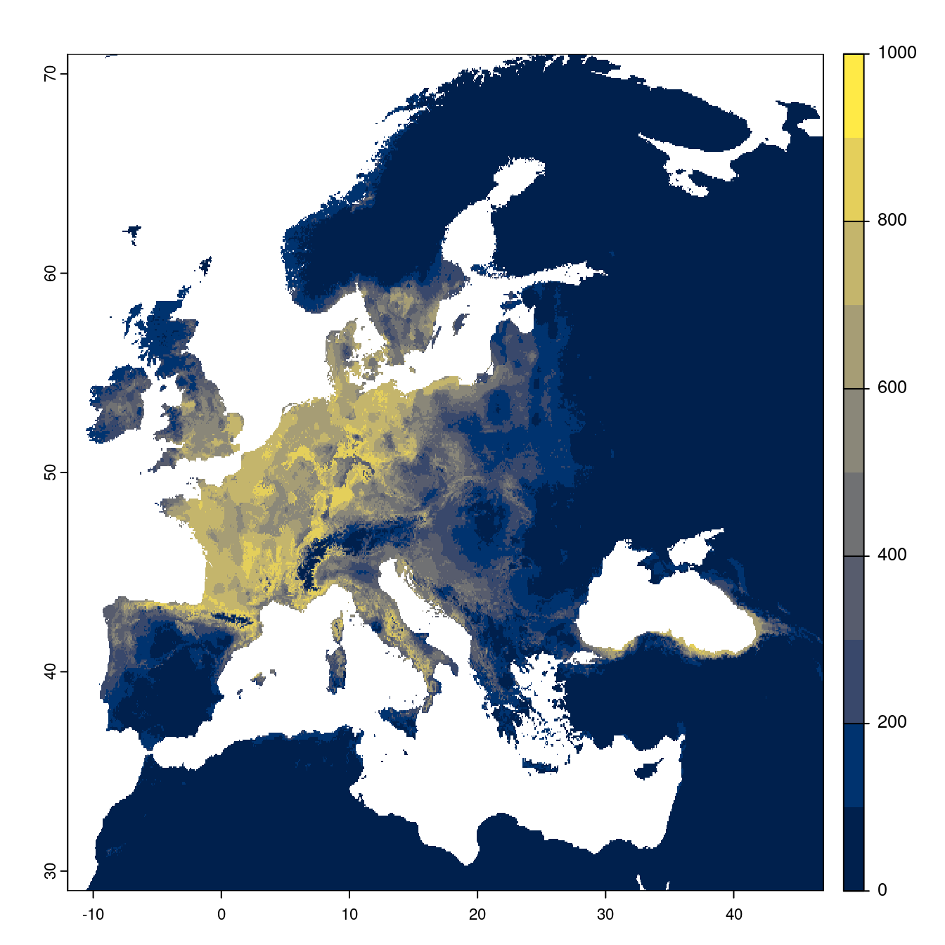
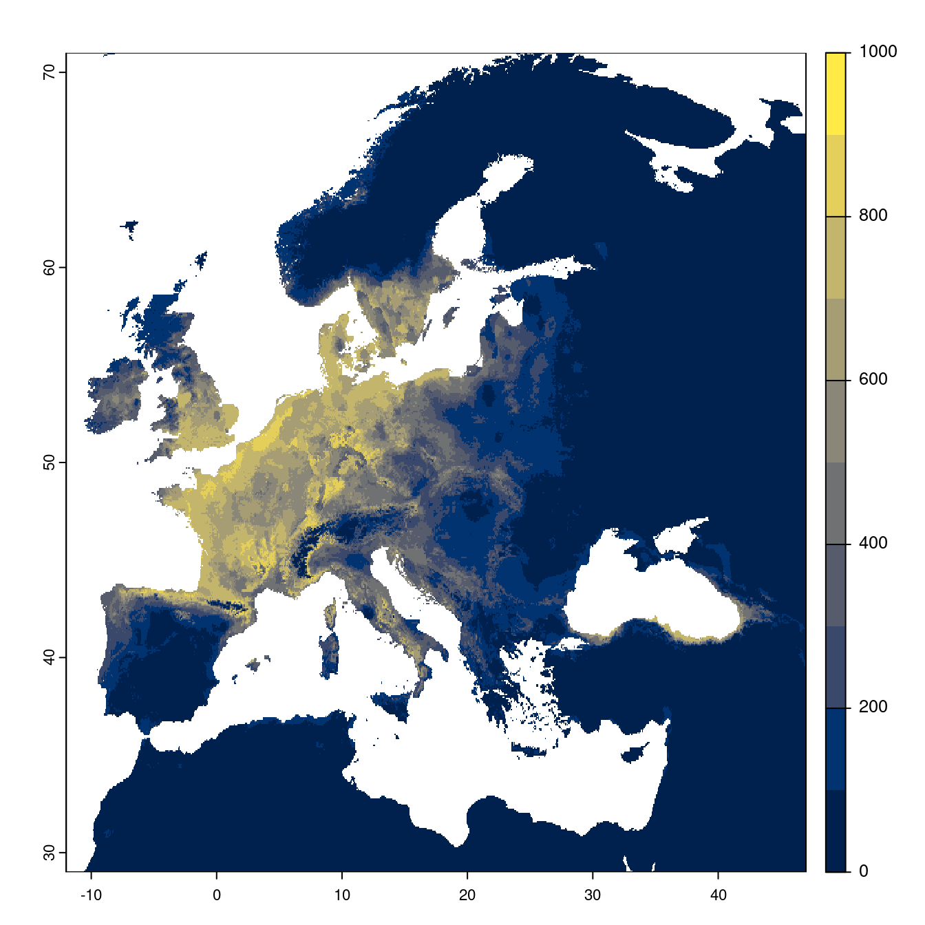
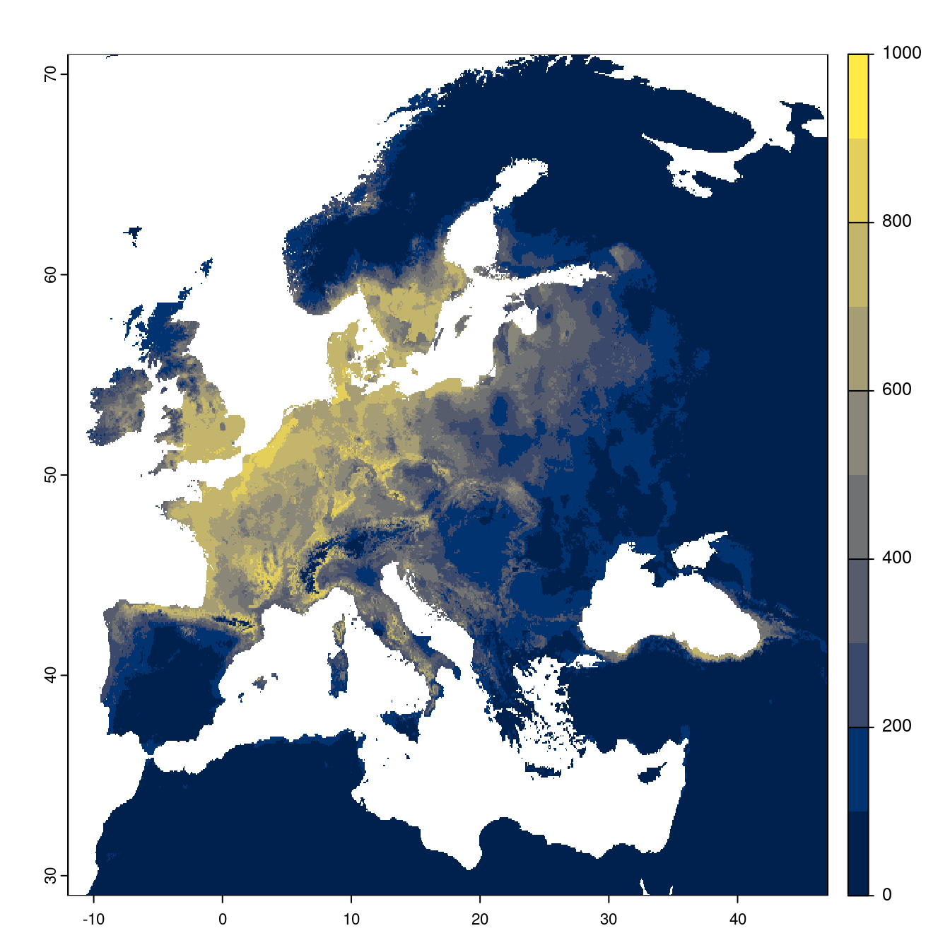

Figure 29.21: Projection des distributions potentielles futures jusqu’à l’horizon 2100 sous le scénario SSP2-4.5 (modèle d’ensemble).
- SSP3-7.0

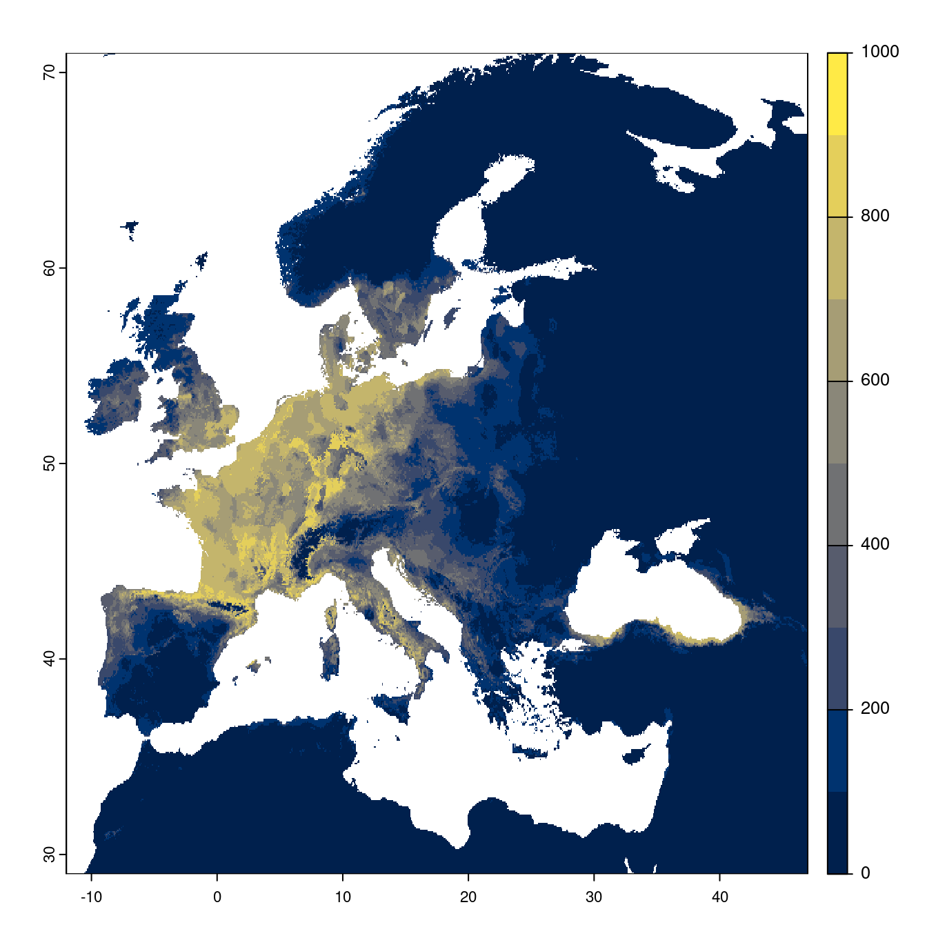

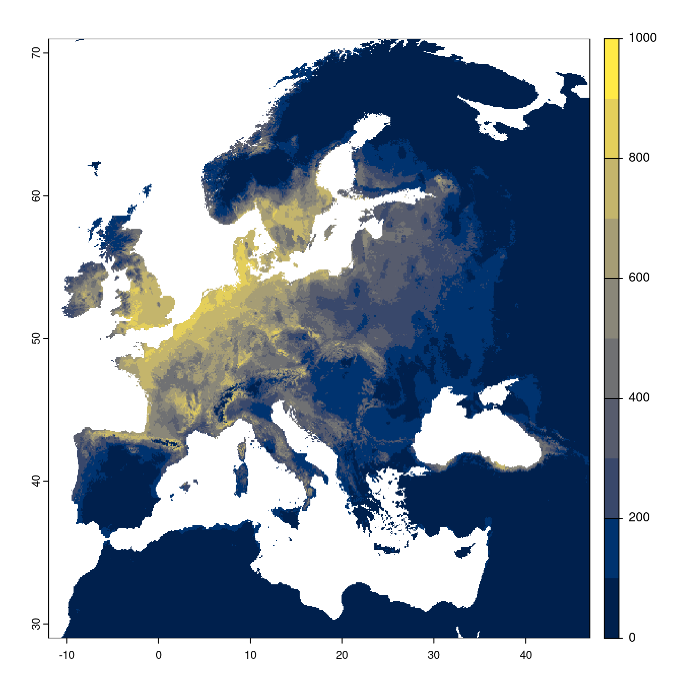
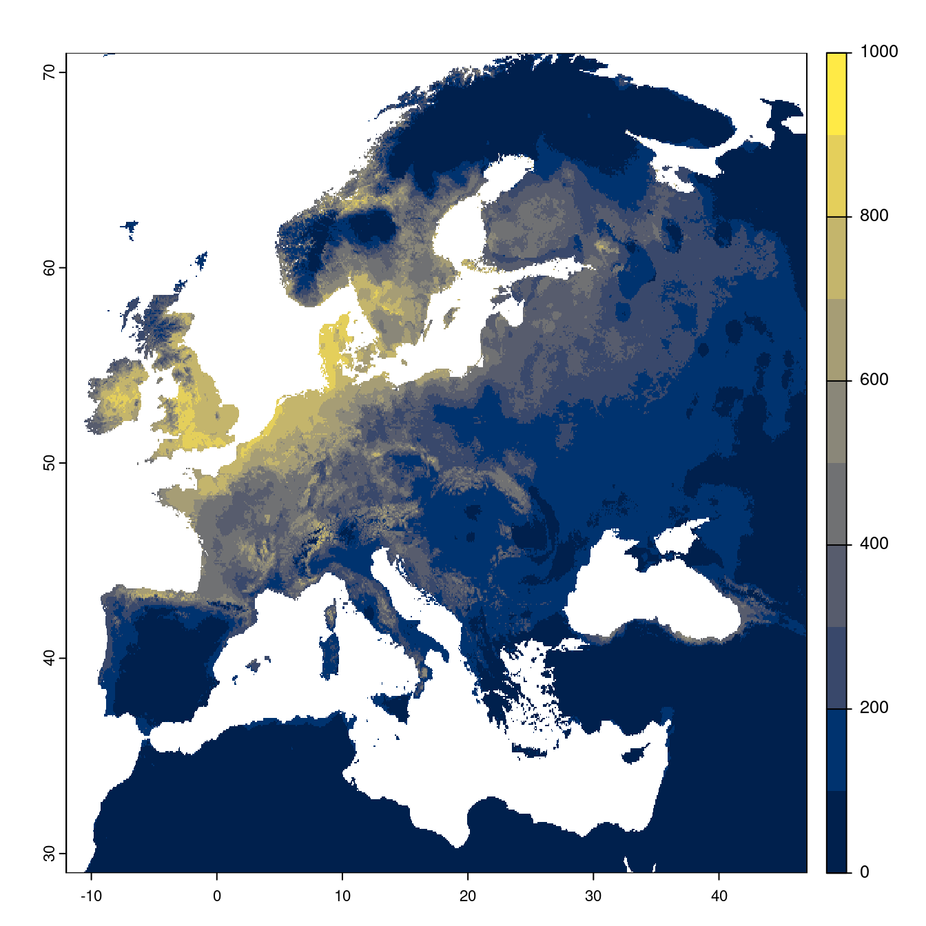
Figure 29.22: Projection des distributions potentielles futures jusqu’à l’horizon 2100 sous le scénario SSP3-7.0 (modèle d’ensemble).
- SSP5-8.5


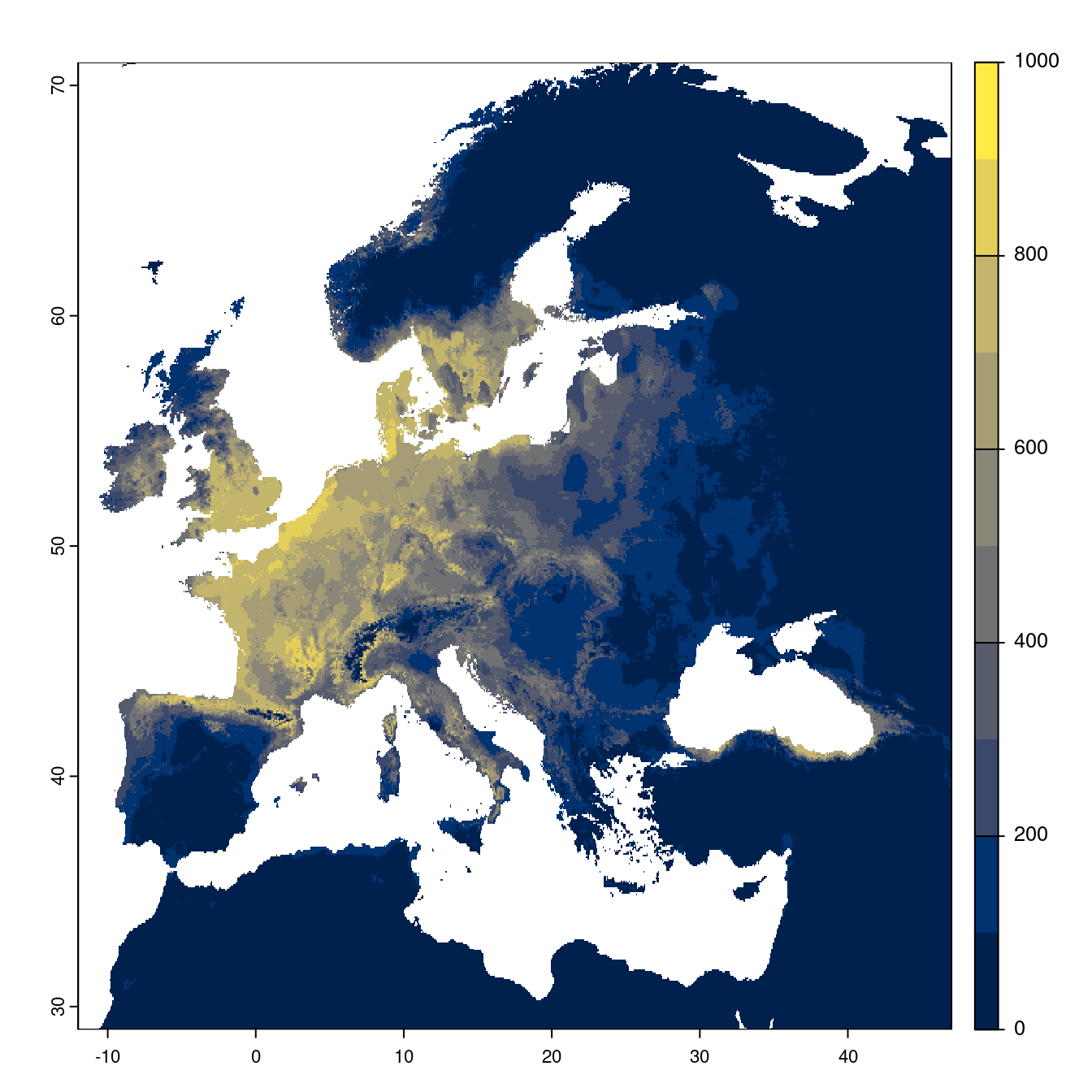
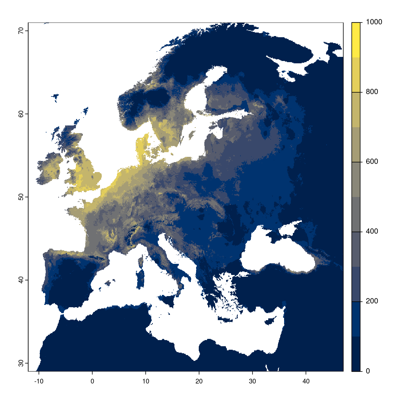
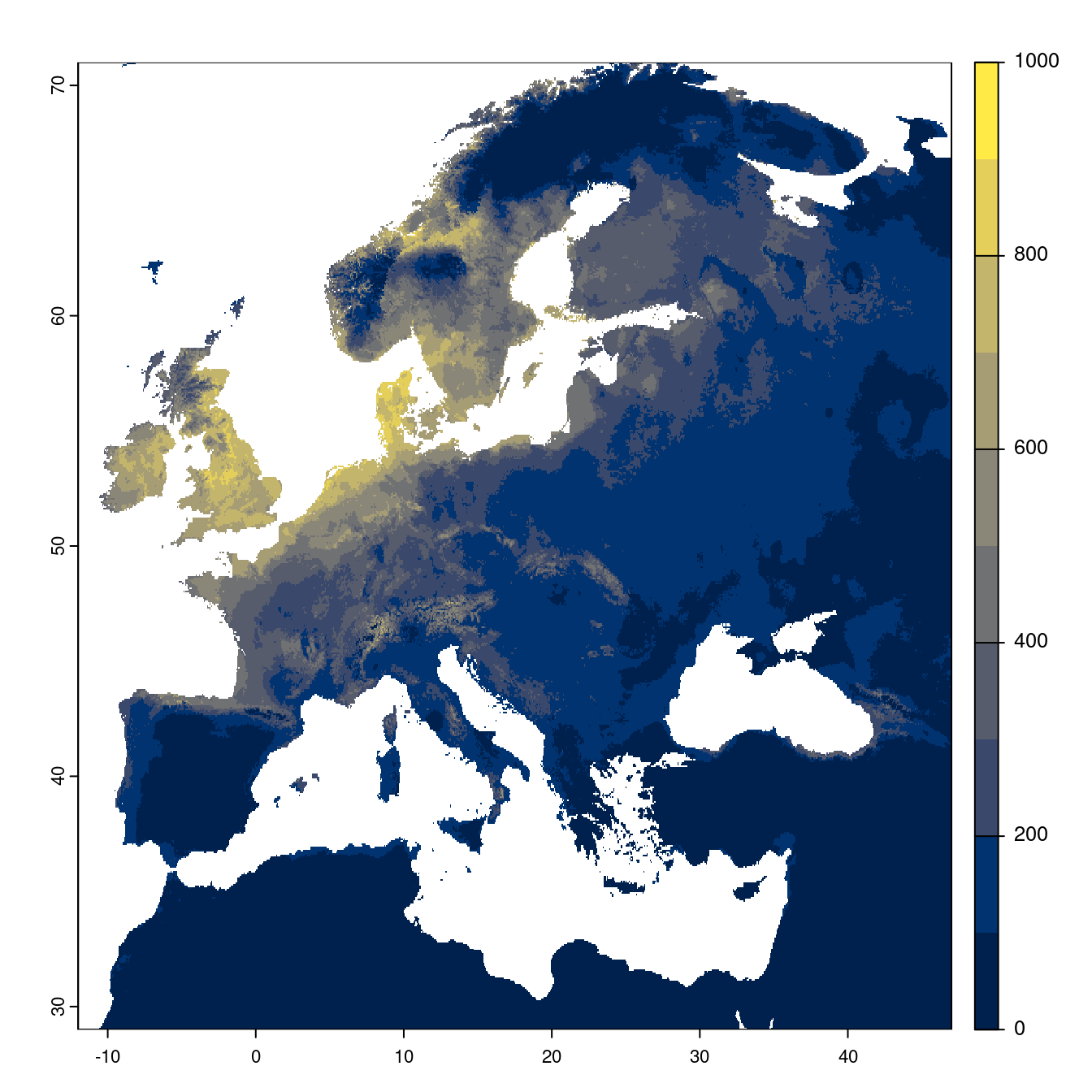
Figure 29.23: Projection des distributions potentielles futures jusqu’à l’horizon 2100 sous le scénario SSP5-8.5 (modèle d’ensemble).
29.4 Inférence à l’échelle de la métropole
- Croisement avec températures de surface 2019 (fournie par la métropole)
- → conditions climatiques favorables à fine échelle
- à peu près 7 pixels × 9 (WorldClim)
29.4.1 Distributions potentielles futures
Même chose que précédemment mais sur les rasters de Grenoble
- SSP1-2.6

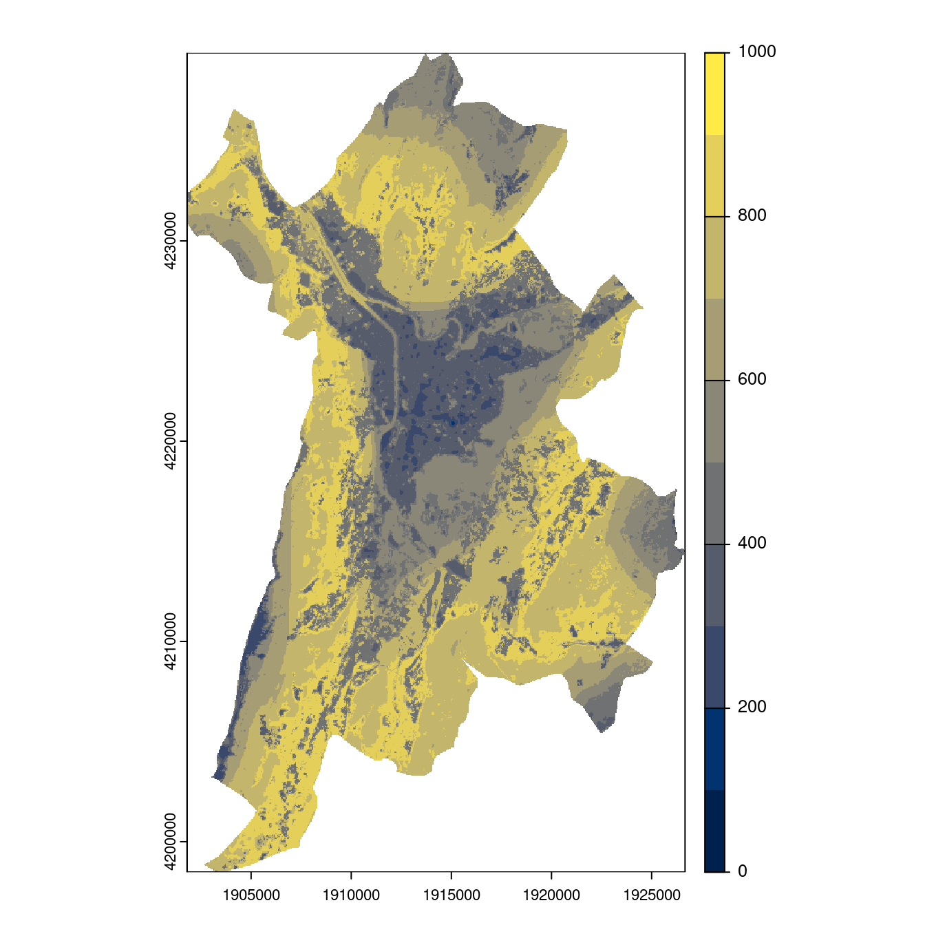
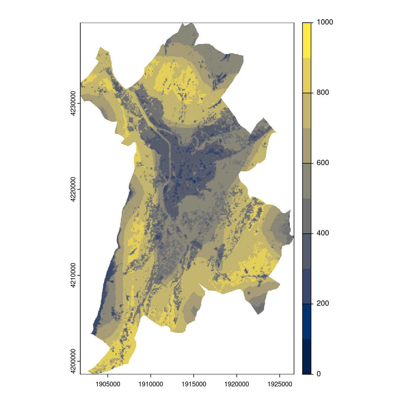
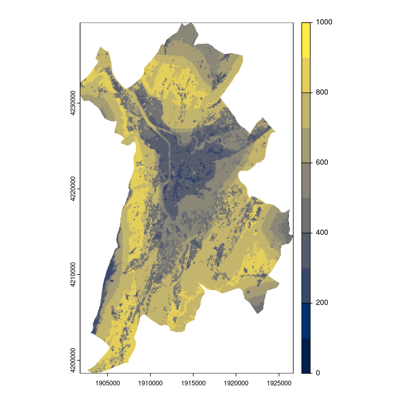
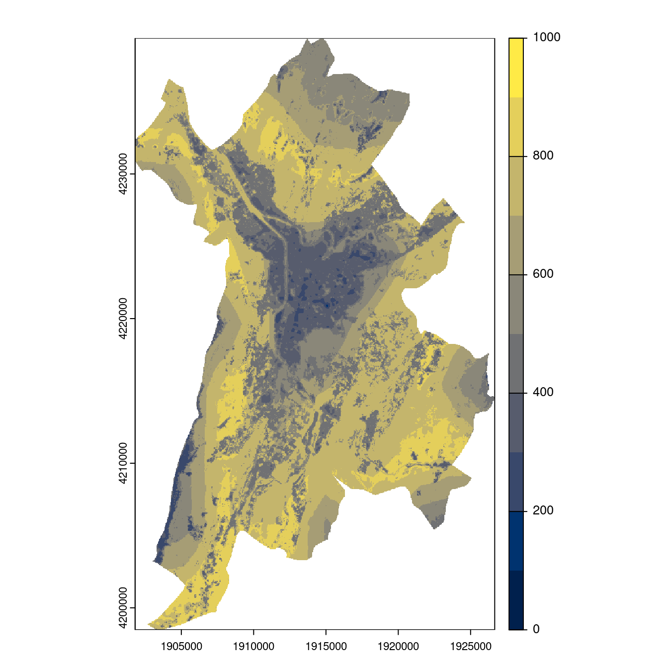
Figure 29.24: Projection des distributions potentielles contemporaine et futures jusqu’à l’horizon 2100 sous le scénario SSP5-8.5 (modèle d’ensemble, GCM IPSL).
- SSP2-4.5

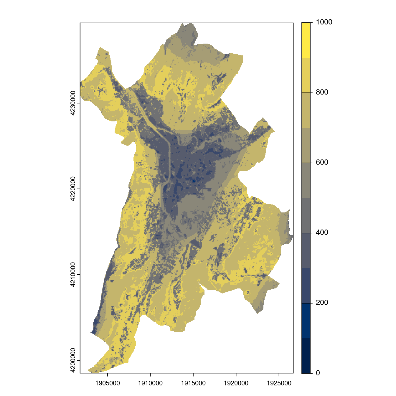
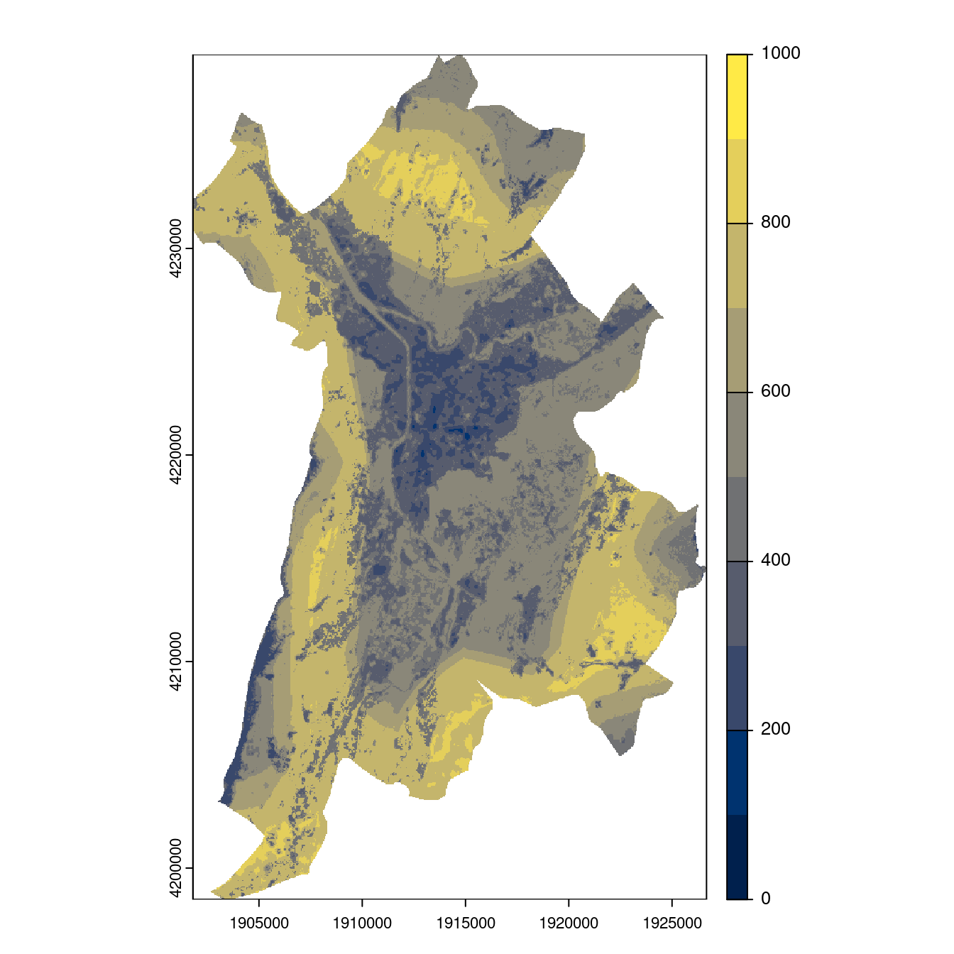
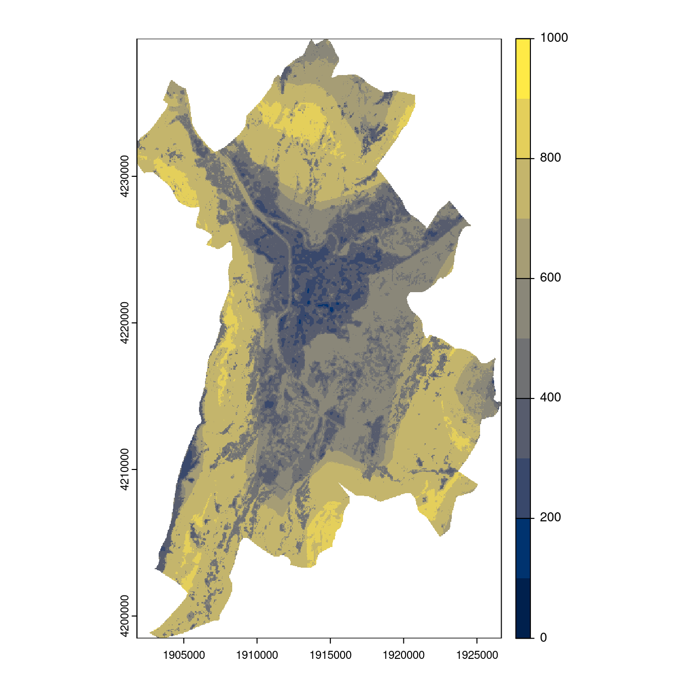
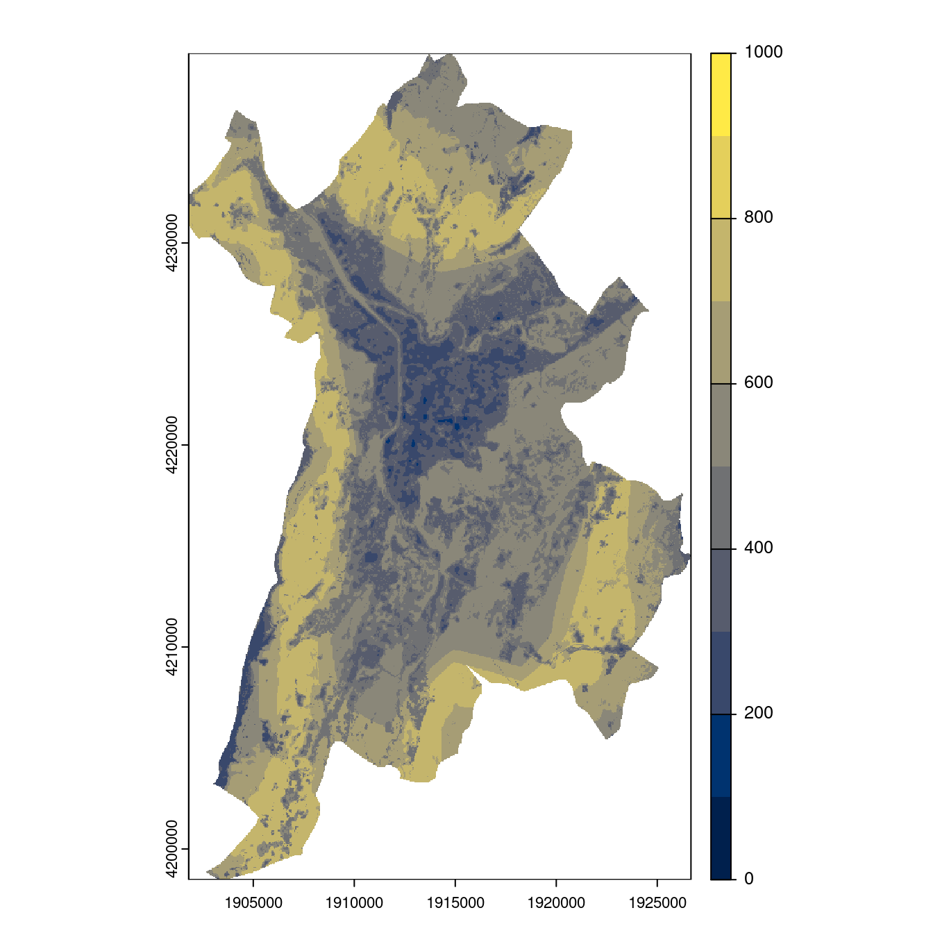
Figure 29.25: Projection des distributions potentielles contemporaine et futures jusqu’à l’horizon 2100 sous le scénario SSP5-8.5 (modèle d’ensemble, GCM IPSL).
- SSP3-7.0

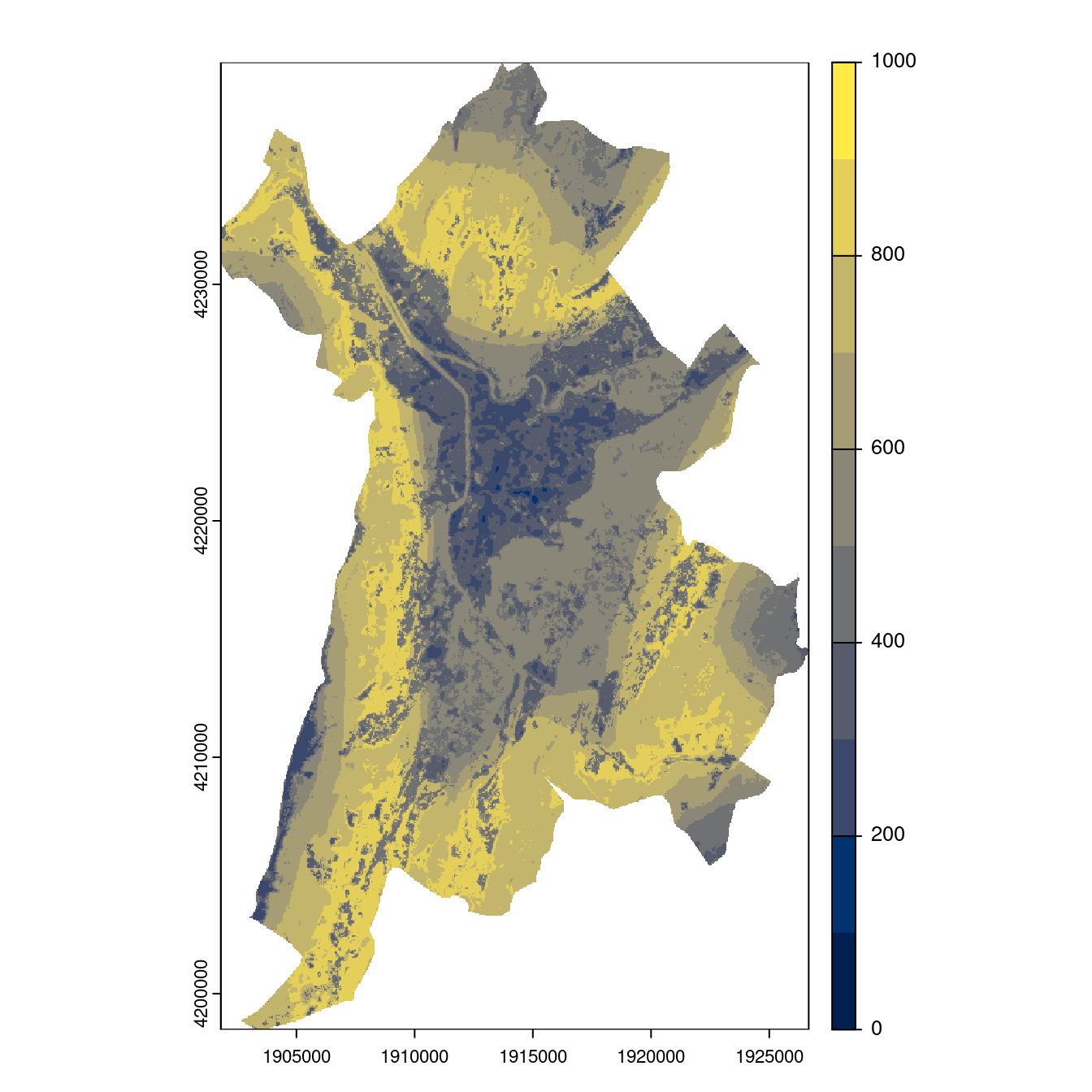
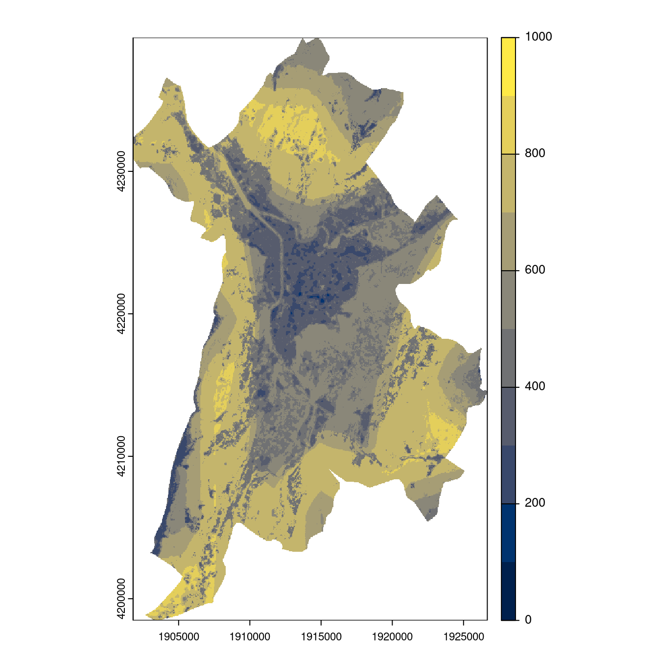
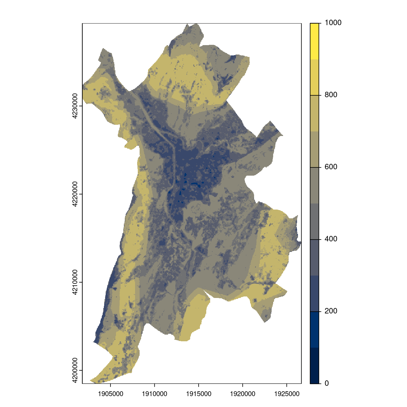
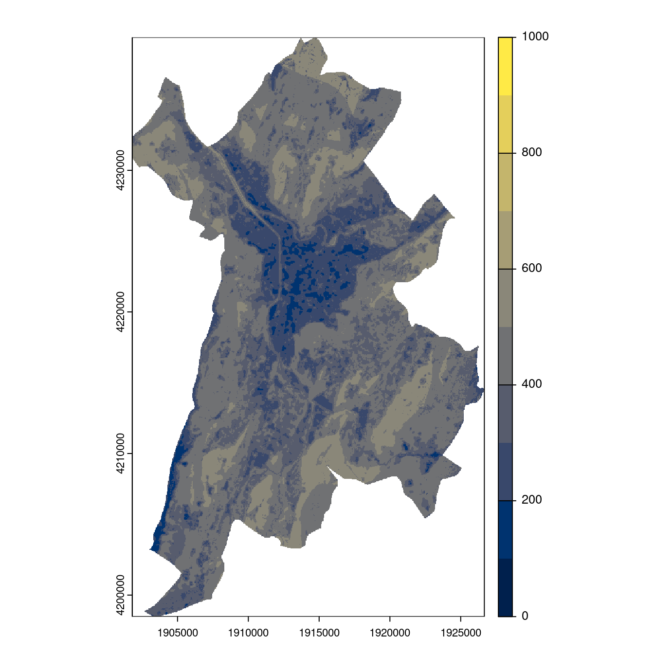
Figure 29.26: Projection des distributions potentielles contemporaine et futures jusqu’à l’horizon 2100 sous le scénario SSP5-8.5 (modèle d’ensemble, GCM IPSL).
- SSP5-8.5
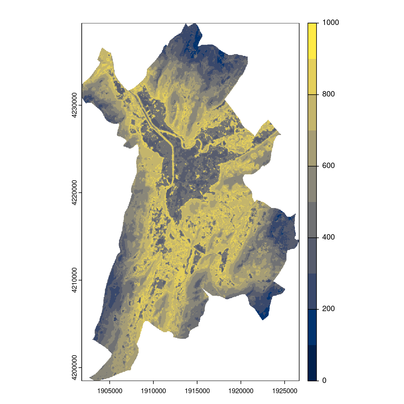
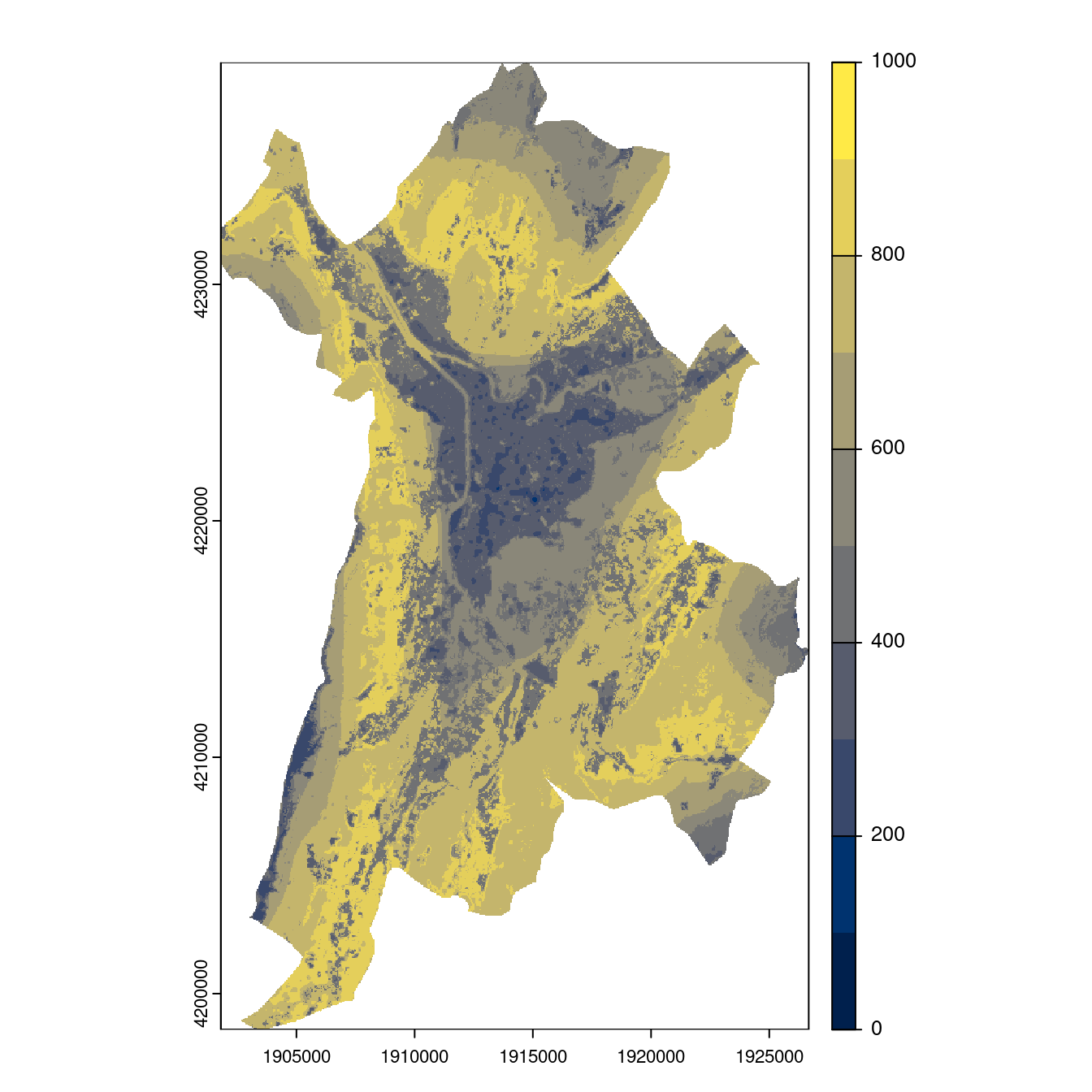
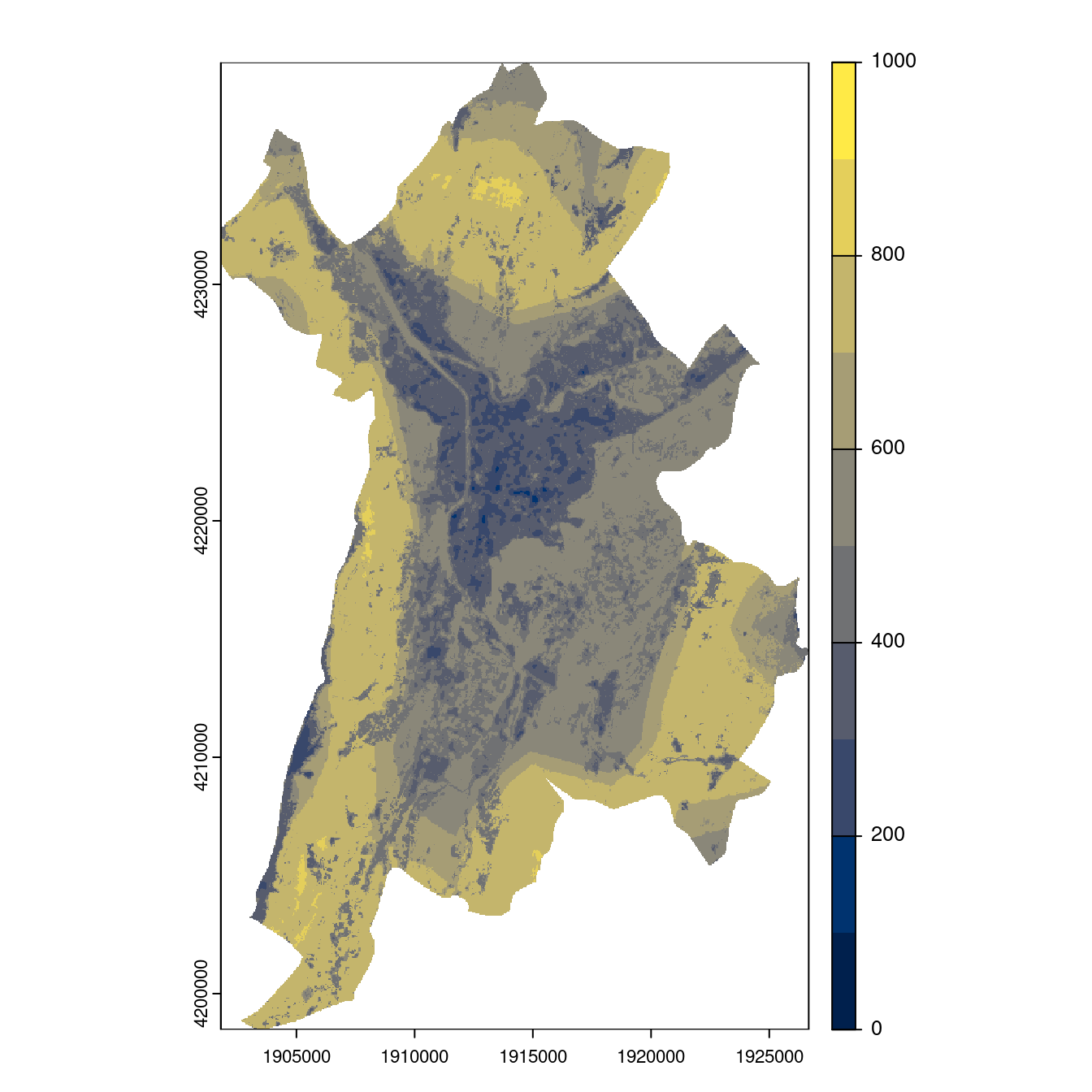
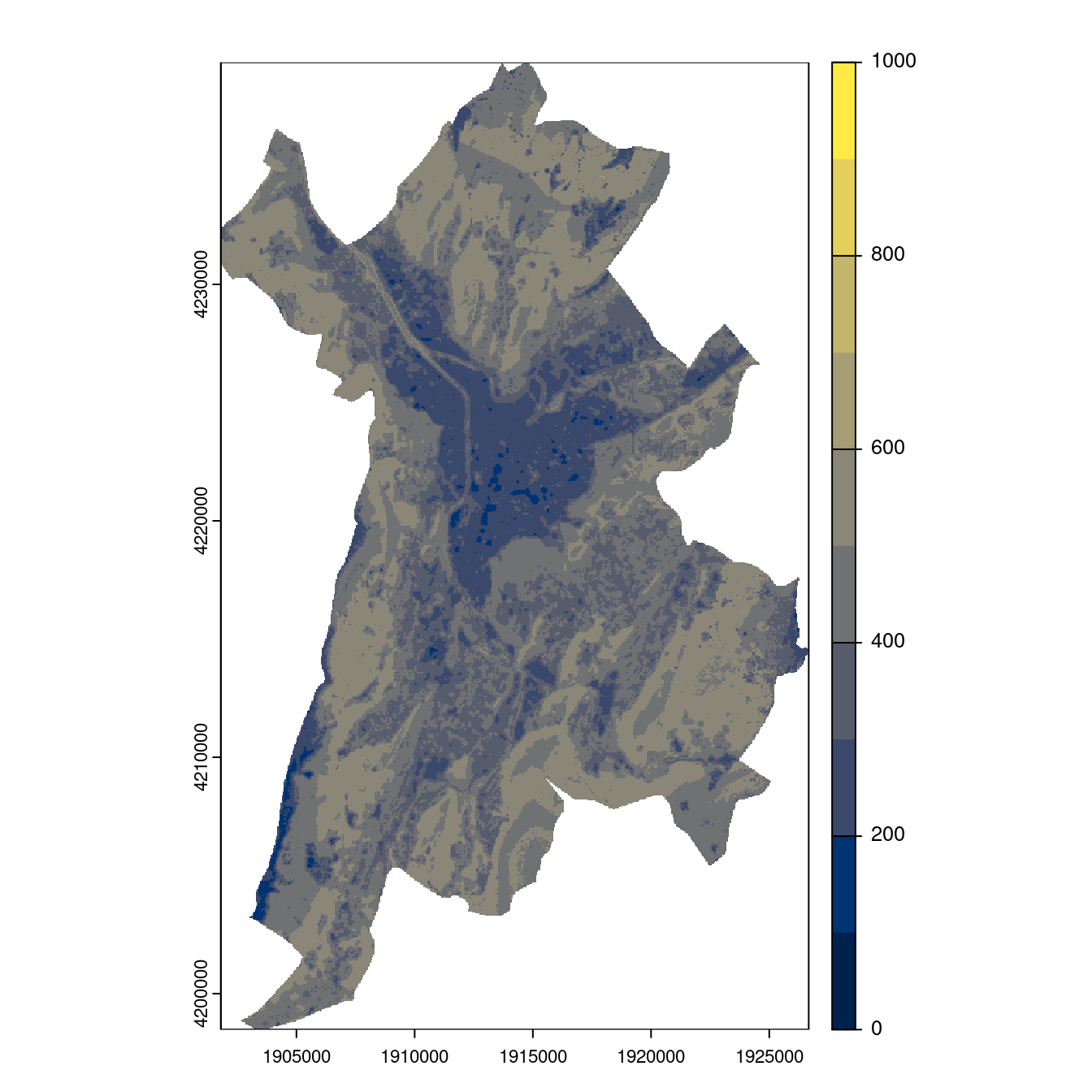
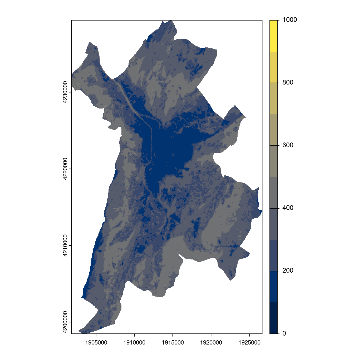
Figure 29.27: Projection des distributions potentielles contemporaine et futures jusqu’à l’horizon 2100 sous le scénario SSP5-8.5 (modèle d’ensemble, GCM IPSL).
29.4.2 Évolution temporelle
# A tibble: 17 × 8
   min         q1          median      mean        q3          max   ssp    year
   <table[1d]> <table[1d]> <table[1d]> <table[1d]> <table[1d]> <tab> <fct> <dbl>
 1 115         443.00      600         583.1888    734         849   0      2000
 2 191         501.00      696         640.5754    784         848   126    2040
 3 190         486.00      638         616.8014    770         845   126    2060
 4 190         489.00      692         635.3581    780         843   126    2080
 5 192         511.00      675         636.6735    771         844   126    2100
 6 191         515.00      748         659.4429    790         848   245    2040
 7 172         451.00      575         584.9202    756         839   245    2060
 8 171         458.00      602         598.1059    752         831   245    2080
 9 170         430.25      557         545.2404    680         787   245    2100
10 174         471.00      622         608.8077    769         842   370    2040
11 173         471.00      601         600.7822    752         837   370    2060
12 169         416.00      548         531.7756    674         797   370    2080
13 156         338.00      419         397.8707    465         589   370    2100
14 190         494.00      691         634.7274    779         845   585    2040
15 170         451.00      570         579.6449    730         816   585    2060
16 165         354.00      443         422.1057    503         604   585    2080
17 138         242.00      338         318.3238    393         539   585    2100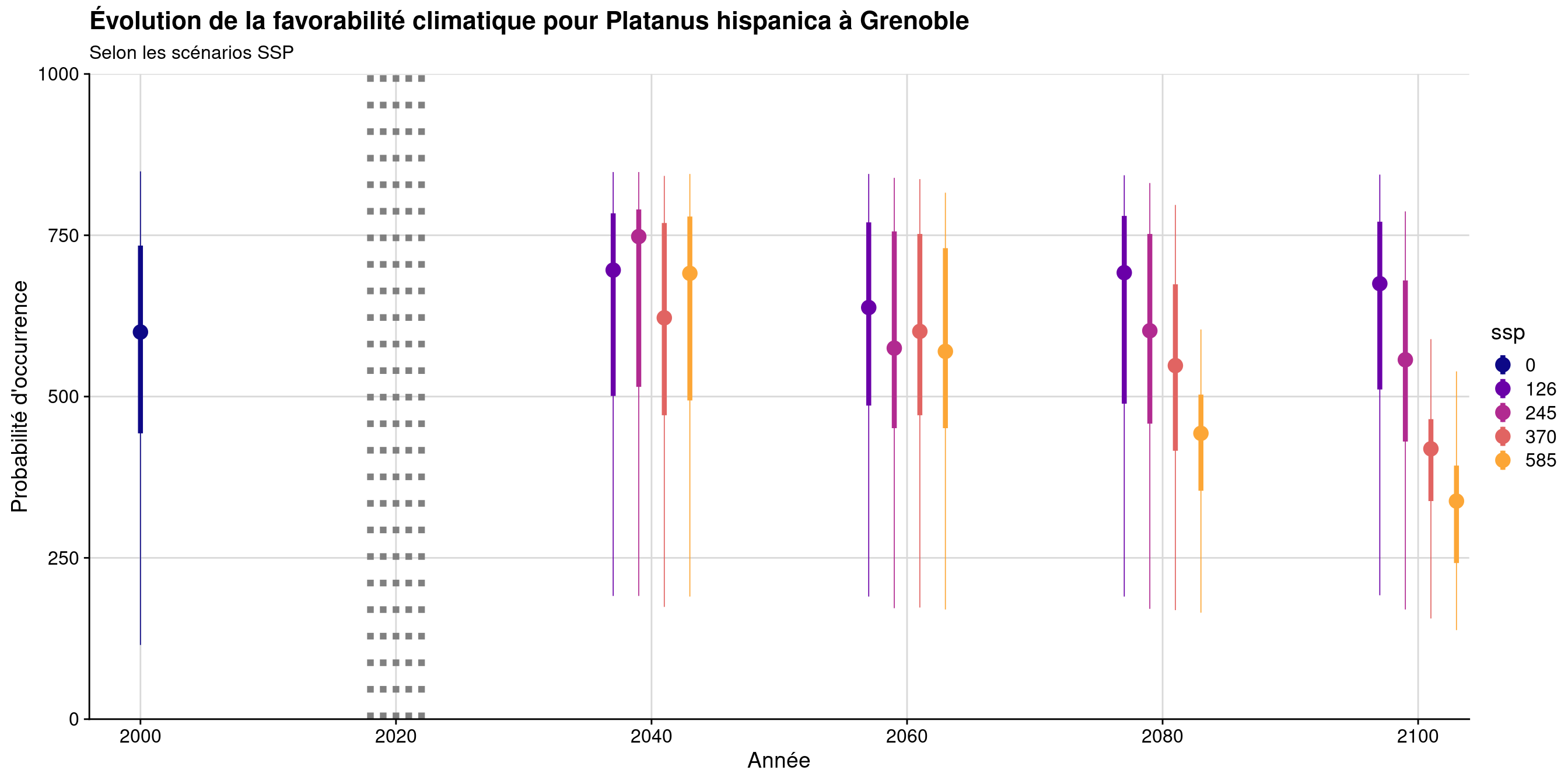
Figure 29.28: Évolution de la favorabilité climatique au cours du XXIème siècle. Le point représente la médiane sur l’étendue de la métropole (i.e. tous les pixels de la carte) ; le trait gras représente 50 % des données intermédiaires (espace inter-quartile) ; le trait fin représente le reste des données du minimum au maximum.